Hello! Welcome to your fourth lesson in the Theory of Computation.
In our last session, you learned how to construct state transition diagrams, the visual blueprints for both DFAs and NFAs. We saw that while DFAs require a complete and unambiguous path for every input, NFAs offer a more flexible, "guess-and-check" design approach.
Today, we will bring those static diagrams to life. Our goal is to trace the execution of both DFAs and NFAs on input strings to determine acceptance or rejection. This lesson bridges the gap between the design of a machine and its dynamic computational process. You will learn to simulate these machines step-by-step, understanding precisely how they decide whether a string belongs to their language.
1. Tracing a Deterministic Finite Automaton (DFA)
The defining characteristic of a DFA is its determinism: for any given state and input symbol, there is exactly one next state. This means tracing a DFA is straightforward, as there is only a single computational path to follow.
The Intuitive Approach: Following the Path
The simplest way to trace a DFA is to start at the initial state and follow the arrows corresponding to the symbols in the input string, one by one.
Let's watch a clear, practical demonstration of this process. The following video first designs a DFA and then traces two different input strings through it, showing how one is accepted and the other is rejected.
Deterministic Finite Automata (Example 1)
This video from Neso Academy provides an excellent walkthrough of tracing a DFA. It will solidify the process of moving from state to state based on input.
Watch from 05:58 to 09:16. First, observe the trace for the string '001', which leads to an accept state. Then, see how the string '101' is traced to a non-accepting 'trap' state, leading to rejection.
As you saw, the process is:
- Start at the initial state.
- For each symbol in the input string (from left to right), follow the transition arrow labeled with that symbol to the next state.
- After reading the last symbol, check your current state.
- If the final state is an accept state (double circle), the string is accepted. Otherwise, it is rejected.
The Formal Approach: The Extended Transition Function
To formalize this process, we introduce the extended transition function, denoted as . While the regular transition function, , tells us the next state after reading a single symbol, tells us the final state after reading an entire string.
The following text from a University of Waterloo lecture note formalizes this tracing process. It introduces the recursive definition of the extended transition function, which is the mathematical foundation for DFA computation.
Read the section titled 'Formally defining what a DFA accepts'. Focus on the recursive definition of δ*. It's defined in two parts: a base case for the empty string (ε), and a recursive step for a string 'xc'.
The definition of is as follows:
- Base Case:
- Reading no symbols leaves the machine in its current state, .
- Recursive Step:
- To find the state after reading string (where is a string and is a symbol), you first find the state after reading (which is ) and then apply the standard transition function for the final symbol .
A DFA accepts a string if and only if .
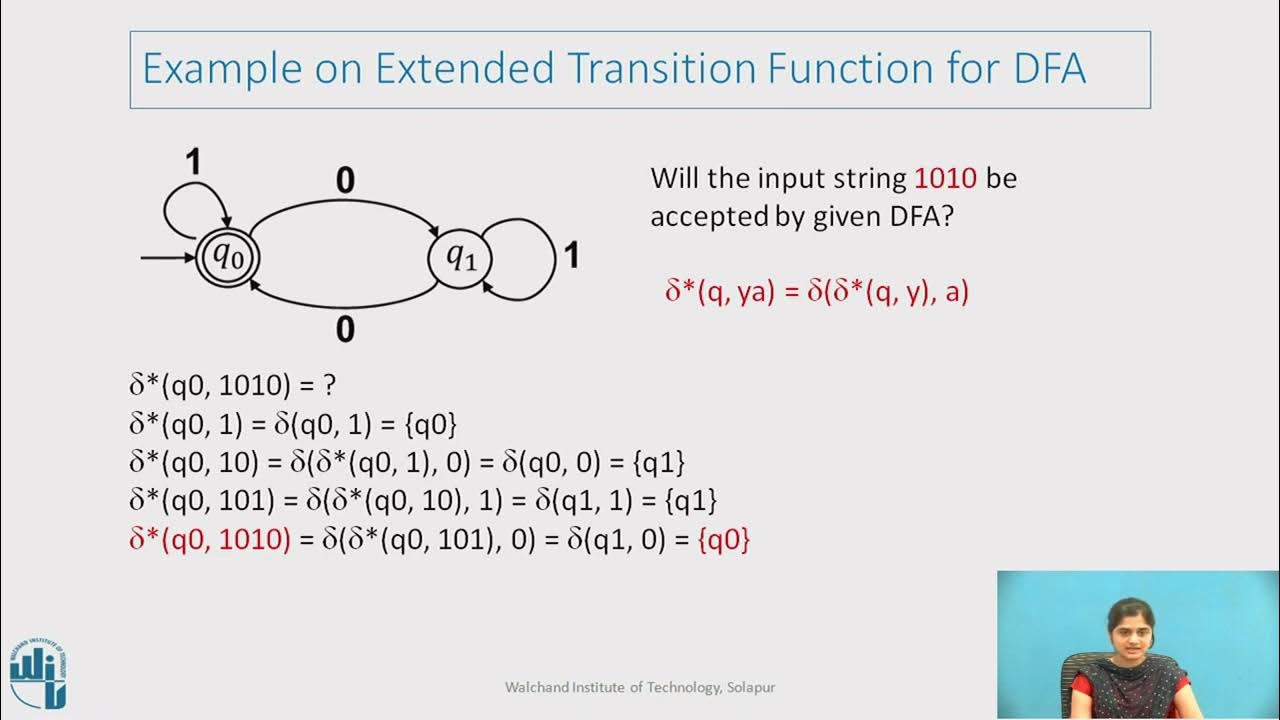
Test your understanding!
Consider the DFA you designed in the last lesson for strings with an even number of 0s. It has two states: (start, accept) and (non-accept).
Trace the input string "10110".
- What is the sequence of states visited?
- Is the string accepted or rejected?
Show answer
-
Sequence of states:
- Start at .
- Read '1': . Current state: .
- Read '0': . Current state: .
- Read '1': . Current state: .
- Read '1': . Current state: .
- Read '0': . Final state: .
The sequence is .
-
Result: The final state is , which is an accept state. Therefore, the string "10110" is accepted. This makes sense, as it contains two 0s (an even number).
2. Tracing a Nondeterministic Finite Automaton (NFA)
Tracing an NFA is fundamentally different. Due to nondeterminism, an NFA can be in a set of multiple states at once. When it reads a symbol, it follows all possible transitions from its current set of states to compute a new set of states. This is akin to exploring multiple computational paths in parallel.
The process of tracing an NFA involves tracking this evolving set of "active" states.
The Core Idea: Tracking Sets of States
The following document from NJIT provides a very clear, table-based method for tracing an NFA. This structured approach helps manage the complexity of multiple parallel paths.
Read the sections 'Nondeterminism' and the two following slides (pages 1-37 to 1-40). Pay close attention to the table on page 1-40 that traces the input string '010110'. Notice how the 'current set of states' is updated after each symbol is read, incorporating ε-transitions along the way.
The key steps for tracing an NFA are:
- Start with a set of states containing just the initial state, . Then, add all states reachable from using only -transitions. This is your initial set of active states.
- For each symbol in the input string:
a. For every state in the current active set, find all possible next states using the standard transition function for the current input symbol.
b. Combine all these next states into a new set.
c. For every state in this new set, add all states reachable from them using only -transitions. This final set is your new set of active states. - After reading the last symbol, look at the final set of active states.
- If this final set contains at least one accept state (i.e., the intersection of your final set and the set of all final states is not empty), the string is accepted. Otherwise, it is rejected.
The Formal Approach for NFAs
Like with DFAs, we can formalize this process with an extended transition function, . For NFAs, maps a state and a string to a set of states. Its definition is more involved because it must handle -transitions and sets of states.
The video below provides a rigorous, step-by-step application of the formal definition to trace an NFA. While the narration includes another language, the on-screen mathematics and diagrams are in English and are exceptionally clear.
Theory of Computation: Extended Transition Function for NFA with an Example
This video by Anita R shows the formal computation of an NFA's execution on the input '1010'. It meticulously builds up the set of reachable states for each prefix of the string.
Watch from 04:40 to 15:40. The core of the video is the step-by-step calculation. Follow along as the instructor computes: δ*(q₀, '1') δ*(q₀, '10') δ*(q₀, '101') δ*(q₀, '1010') Finally, observe how the result is checked against the set of final states to determine acceptance.
The NFA acceptance condition can be stated formally: An NFA accepts a string if and only if .
Conclusion
Today you learned how to execute, or "run," finite automata on input strings. This is the heart of what these machines do: they are computational devices for answering the question, "Is this string in the language?"
Key Takeaways:
- DFA Tracing: Follows a single, deterministic path. The machine is in exactly one state at any time. A string is accepted if this single path ends in an accept state. This can be formalized with the extended transition function .
- NFA Tracing: Involves tracking an evolving set of possible states. The computation effectively branches, and we follow all paths in parallel. This process must also account for -transitions.
- NFA Acceptance: A string is accepted if the final set of active states contains at least one accept state.
Preview of the Next Lesson:
We've now seen that NFAs are often simpler to design, but their execution model (tracking sets of states) is more complex than a DFA's simple path. DFAs are simpler to execute but can be much more complex to design. This presents a trade-off. In the next lesson, we will resolve this by learning the subset construction algorithm, a powerful technique to convert any NFA into an equivalent DFA. This process formalizes the very tracing procedure you learned today for NFAs.