DFA and NFA State Transition Diagrams

Hello! Welcome to your third lesson.

In the previous lesson, we established the formal 5-tuple "blueprints" for Deterministic and Nondeterministic Finite Automata. We saw that the crucial difference lies in their transition functions: a DFA's transition function maps to a single state, while an NFA's maps to a set of states, allowing for multiple possibilities.

Today, we'll bring these abstract definitions to life. The learning outcome is to construct state transition diagrams for DFAs and NFAs to represent language acceptors. These diagrams are the primary tool computer scientists use to visualize, design, and reason about these computational models. You'll learn the conventions for drawing them and the different design philosophies for DFAs and NFAs.

1. The Anatomy of a State Transition Diagram

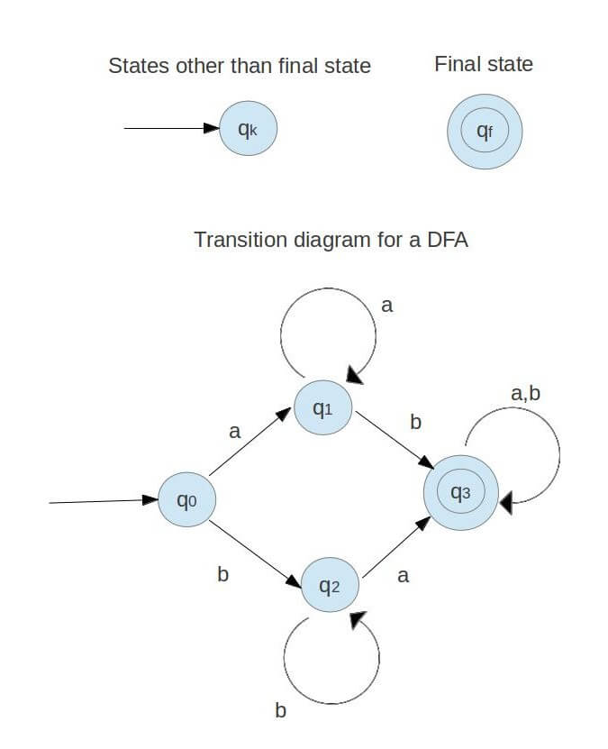
A state transition diagram is a directed graph with specific conventions. Mastering these conventions is the first step to building and understanding automata.

States ( $Q$ ): Represented by circles (vertices).
Start State ( $q_{0}$ ): Indicated by an incoming arrow with no source state.
Accept/Final States ( $F$ ): Indicated by a double circle. A machine can have zero, one, or multiple accept states.
Transitions ( $δ$ ): Represented by directed edges between states. Each edge is labeled with the input symbol(s) from the alphabet $Σ$ that trigger that transition.

DFA State Transition Diagram Conventions and Example — This image illustrates the standard graphical conventions for a state transition diagram. It shows a start state (q0), non-final states (q1, q2), a final state (q3), and transitions labeled with input symbols 'a' and 'b'.

2. Constructing Diagrams for DFAs

When designing a DFA, you must adhere to its deterministic nature. From every state, there must be exactly one outgoing transition for every symbol in the alphabet. This ensures there's always a single, unambiguous computational path.

The Thought Process: States as Memory

The key to designing a DFA is to think of each state as "remembering" a crucial piece of information about the prefix of the string processed so far.

Let's see this in action. The following video builds a DFA for a "heatwave detector" and provides an excellent intuitive walkthrough of the design process.

Regular Languages: Deterministic Finite Automaton (DFA)

This video from the 'lydia' channel demonstrates how to construct a DFA from a simple problem description. Pay attention to how each state represents a specific condition (e.g., 'no hot days yet' or 'one consecutive hot day').

Watch from 01:01 to 03:54. Observe how the diagram is built step-by-step and how the states q0, q1, and q2 correspond to the progress made toward detecting a heatwave.

As the video showed, the states represent the memory of the machine:

q0: The initial state. We haven't seen any consecutive hot days (1s).
q1: We have seen one consecutive hot day.
q2: We have seen two consecutive hot days. This is an accept state.

Notice that from q0, if we see a '0', we stay in q0. If we're in q1 and see a '0', the streak is broken, so we go back to q0.

The Trap State

What happens if the input sequence can no longer lead to an accepted string? A DFA must still have a transition defined. We handle this with a trap state (or dead state)—a non-accepting state from which there is no escape. Once the machine enters a trap state, it will remain there for all subsequent inputs.

Consider the language of all strings over $Σ = {a, b}$ that are formed by one or more repetitions of "ab" (i.e., L = {ab, abab, ...}).

DFA for (ab)+

Figure 3.1 from the provided UPenn lecture notes. This DFA accepts the language L = {ab}+. State 3 is a trap state. If the string deviates from the 'ab' pattern (e.g., 'aa' or 'aba'), the machine enters state 3 and can never reach the accept state 2.

Test your understanding!

Design a state transition diagram for a DFA that accepts all strings over $Σ = {0, 1}$ containing an even number of 0s. (An even number can be zero.)

Show answer

You only need two states:

q_even (start and accept state): Represents having seen an even number of 0s.
q_odd (non-accept state): Represents having seen an odd number of 0s.

The diagram would look like this:

Start at q_even. Since zero is an even number, this is also a final state.
From q_even:
- On input '1', stay in q_even (the count of 0s doesn't change).
- On input '0', move to q_odd.
From q_odd:
- On input '1', stay in q_odd.
- On input '0', move back to q_even.

3. Constructing Diagrams for NFAs

Designing NFAs is often more intuitive because you don't need to specify transitions for every symbol from every state. You only need to define the paths that lead to acceptance. This is like outlining the "success" scenarios, while any undefined transition implicitly leads to a "death" for that computational path.

This "guess-and-check" nature makes NFAs particularly good for languages defined by substrings or positional properties.

The following video provides a fantastic series of examples.

NFA Examples || Non Deterministic Finite Automata || Theory of Computation || TOC || FLAT

This video from Sudhakar Atchala walks through constructing NFAs for several common language patterns. It's a very practical, example-driven tutorial.

Watch the examples for strings 'starting with 01' (00:17-02:54), 'ending with 01' (02:54-05:28), 'containing substring 01' (05:28-06:51), and where the 'third symbol from the right end is a' (06:51-08:46). Notice how simple and direct the constructions are.

Let's summarize the design pattern for a substring, like "all strings containing 01":

Initial state (q0): A self-loop for 0,1. This allows the machine to skim over any characters before the substring begins.
Middle path: A transition on 0 from q0 to q1, and a transition on 1 from q1 to q2. This path recognizes the substring itself.
Final state (q2): A self-loop for 0,1. This allows the machine to accept the string even if there are characters after the substring.

NFA vs. DFA: Simplicity vs. Completeness

The power of NFA design is most apparent when you compare it to the DFA for the same language.

Comparison of NFA and DFA State Transition Diagrams — This image compares the NFA and DFA for the language of all strings containing '11'. The NFA (top) is simple and directly models the search for '11'. The DFA (bottom) is more complex, as it must explicitly define what to do in every situation, including transitions to a trap state (q3).

NFA with $ϵ$ -Transitions

As we saw in the last lesson, NFAs can also have $ϵ$ -transitions, which allow the machine to change state without consuming an input symbol. These are a powerful tool for combining smaller machines or representing choice.

For example, let's design an NFA for the language of strings that contain either the substring ab or the substring ba. We can design two separate NFAs—one for ab and one for ba—and then "glue" them together from a new start state using $ϵ$ -transitions.

An NFA that accepts any string containing the substring 'ab' or 'ba'. The automaton starts in q0 and, without consuming any input, can jump to either the machine that looks for 'ab' (starting at q1) or the machine that looks for 'ba' (starting at q4).

Test your understanding!

Draw the state transition diagram for an NFA that accepts all strings over $Σ = {a, b}$ that end with 'a'.

Show answer

This is a classic NFA design.

q0 (start state): This state represents "we are not sure if we are at the end of the string yet". It has a self-loop on both 'a' and 'b'. This allows it to read any sequence of characters. There is also a transition from q0 to itself on input 'a', which represents one of the "guesses" for the final 'a'.
q1 (accept state): This state represents the guess that "the character we just read might be the last one".

The transitions are:

From q0, on input 'a' or 'b', transition to q0.
From q0, on input 'a', also transition to q1.

When the input string ends, if one of the parallel computation paths is in state q1, the string is accepted. For example, on input "baba":

Path 1: q0 -> q0 -> q0 -> q0 (ends in non-accept state)
Path 2: On the final 'a', a path can also go from q0 to q1. This path ends in an accept state, so "baba" is accepted.

A simpler-looking but equivalent diagram:

q0 (start state): self-loop on 'a', 'b'.
Transition from q0 to q1 on 'a'.
q1 is the accept state with no outgoing transitions.

Conclusion

In this lesson, we moved from the abstract formulas of automata to their visual and practical representation. State transition diagrams are the language we use to design and communicate these simple, yet powerful, computational models.

Key Takeaways:

State diagrams have clear conventions for representing states, transitions, the start state, and accept states.
DFA diagrams must be complete: every state needs exactly one outgoing transition for every symbol in the alphabet. This often requires using a trap state. Their design is methodical, tracking the properties of the string seen so far.
NFA diagrams are often simpler and more intuitive to design. You only need to draw the "success" paths, leveraging nondeterminism to handle choices and "guesses."
$ϵ$ -transitions in NFAs provide a convenient way to model state changes without consuming input, which is especially useful for combining automata.

Preview of the Next Lesson:
We now know how to define automata formally and how to draw them. The next logical step is to see them in action. In the next lesson, we will trace the execution of both DFAs and NFAs on input strings to formally determine whether a string is accepted or rejected. This will connect the static diagrams you built today to the dynamic process of computation.

Recommended resources