CFG Production Rules from PDA Transitions

1. The Formal Construction Algorithm

While our previous lesson's three rule types (A_pp → ε, A_pq → A_pr A_rq, A_pq → a A_{rs} b) are conceptually sound, there is a more direct and mechanical algorithm that is often used in practice. This algorithm uses a different, but equivalent, style of variable.

CFG Variable Definition

The variables (non-terminals) in our new grammar will be of the form [p, A, q], where:

• p and q are states of the PDA.
• A is a stack symbol.

The intuitive meaning of the variable [p, A, q] is:

The language of all input strings w that take the PDA from state p to state q, where the net result of the computation is the consumption of the single symbol A from the top of the stack.

The stack can grow and shrink arbitrarily during the computation for w, but it must end up exactly one symbol shorter than it started.

The Algorithm Steps

Given a PDA P = (Q, Σ, Γ, δ, q₀, Z₀), we construct an equivalent CFG G = (V, T, P, S) as follows:

1. Terminals (T): The terminals of the grammar are the input symbols of the PDA: T = Σ.

2. Variables (V): The variables include a new start symbol S and one variable for every possible triple:
   V = {S} ∪ { [p, A, q] | p, q ∈ Q, A ∈ Γ }.

3. Start Productions: We add productions for the start symbol S of the form:
   $S\to [q_0,Z_0,q]$
   for every state q in Q. This rule captures the overall goal: a string is in the language if it takes the PDA from the start state q₀ to any state q, with the net effect of emptying the stack (i.e., consuming the initial stack symbol Z₀).

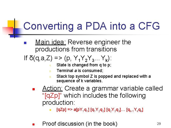
4. Transition Productions: For each transition in the PDA, we generate a set of production rules. Consider a generic transition: δ(p, a, A) = (r, B₁B₂...B_k). This means "in state p, reading input a with A on the stack, go to state r and replace A with the string B₁B₂...B_k".

   • Case 1: Pop (k = 0)
     If the transition is a pop, δ(p, a, A) = (r, ε), the generated rule is simple:
     $[p,A,r]\to a$
     This means: "To go from p to r by consuming A, you can just read input a."

   • Case 2: Push/Replace (k > 0)
     If the transition pushes symbols B₁B₂...B_k, we need to account for the sub-computations that will eventually pop each of these new symbols. The generated rule is:
     $[p,A,q_k]\to a[r,B_1,q_1][q_1,B_2,q_2]...[q_{k-1},B_k,q_k]$
     This rule is created for every possible combination of intermediate states q₁, q₂, ..., q_k from Q. This rule is the heart of the construction. It says:

     "To go from p to q_k consuming A, you can:

     1. Read input a.
     2. This puts you in state r with B₁...B_k on the stack.
     3. Now, find a path from r to some state q₁ that consumes B₁.
     4. Then, find a path from q₁ to q₂ that consumes B₂.
     5. ...and so on, until you find a path from q_{k-1} to q_k that consumes B_k."

This decomposition is what gives the construction its power. The large number of rules generated accounts for the non-determinism of both the PDA and the resulting CFG.

2. A Concrete Example: Step-by-Step Conversion

Let's see this algorithm in action. We'll use a PDA that recognizes the language {a^m b^m | m ≥ 1}.

The following video walks through an almost identical problem. The presenter uses a slightly different notation for variables (e.g., q₀Aq₁ instead of [q₀, A, q₁]), but the logic is precisely the same as the algorithm we just defined.

Let's recap the key points from the video, mapping them to our algorithm:

• Variables and Start Symbol (00:00 - 04:44): The video correctly identifies that the CFG variables are formed from combinations of (state, stack_symbol, state). The start productions S → [q₀, Z₀, q₀] and S → [q₀, Z₀, q₁] are created, setting up the goal of consuming the initial stack symbol Z₀ and ending in any state.

• Two-Symbol Push (04:44 - 11:34): The PDA transition δ(q₀, a, A) = (q₀, AA) pushes two symbols. Our algorithm states this creates rules of the form [q₀, A, q₂] → a [q₀, A, q₁][q₁, A, q₂]. Since there are two states (q₀, q₁), the intermediate state q₁ can be either q₀ or q₁, and the final state q₂ can also be either q₀ or q₁. This gives 2 * 2 = 4 total productions for this single PDA transition, exactly as shown in the video.

• One-Symbol Push (11:34 - 14:48): The PDA transition δ(q₀, b, A) = (q₁, A) replaces one symbol with one other. This is a k=1 push. The rule form is [q₀, A, q₁] → b [q₁, A, q₁]. Since there is only one final state to choose (q₁), and no intermediate states, this generates 2 rules (one for each possible q₁ in {q₀, q₁}), just as shown.

• Pop / Epsilon-Push (14:48 - 17:11): The PDA transition δ(q₁, a, A) = (q₁, ε) is a pop. This is our k=0 case. The rule is [q₁, A, q₁] → a. This is a direct mapping and generates only one production.

Alternative Formalisms

It's worth noting that the algorithm we've studied is not the only one. The conceptual method from our previous lesson (using variables A_pq) is also a valid and powerful construction. The resources below lay out this alternative. You don't need to master it, but it's good to be aware that different, equivalent paths exist to prove the same result.

This alternative method often feels more intuitive but can be harder to apply mechanically. The algorithm we focused on today is less intuitive but is a straightforward, deterministic procedure for generating the grammar. Both arrive at an equivalent CFG.

Conclusion

You have now mastered the formal algorithm for converting any PDA into an equivalent CFG. This is a significant result that completes the proof of equivalence between these two models of computation.

Key Takeaways:

• The conversion is an algorithmic process that translates each PDA transition into one or more CFG production rules.
• The variables of the CFG, [p, A, q], elegantly capture the idea of a "sub-computation" that consumes a specific stack symbol A while transitioning between states p and q.
• The number of rules generated by a single PDA transition depends on the number of symbols it pushes onto the stack and the total number of states in the PDA, reflecting the non-determinism involved.
• While the resulting grammar can be very large and contain many useless or unreachable productions, it is guaranteed to be equivalent to the source PDA. Simplification algorithms can be applied afterward.

Preview of the Next Lesson:
Now that we've established that PDAs and CFGs are equivalent, we'll shift our focus to exploring the limits of this class of languages. We will learn about Deterministic Pushdown Automata (DPDA) and see that, unlike with finite automata, adding nondeterminism to PDAs gives them more power. We will identify specific languages that can be recognized by a nondeterministic PDA but not by any deterministic one.