BFS for Shortest Paths in Unweighted Graphs

1. The Core Idea: Exploring in Layers

At its heart, Breadth-First Search is a systematic way to explore a graph. Starting from a source vertex, it visits all its immediate neighbors first. Then, for each of those neighbors, it visits their unvisited neighbors, and so on. This creates a "layer-by-layer" or "ripples-in-a-pond" effect.

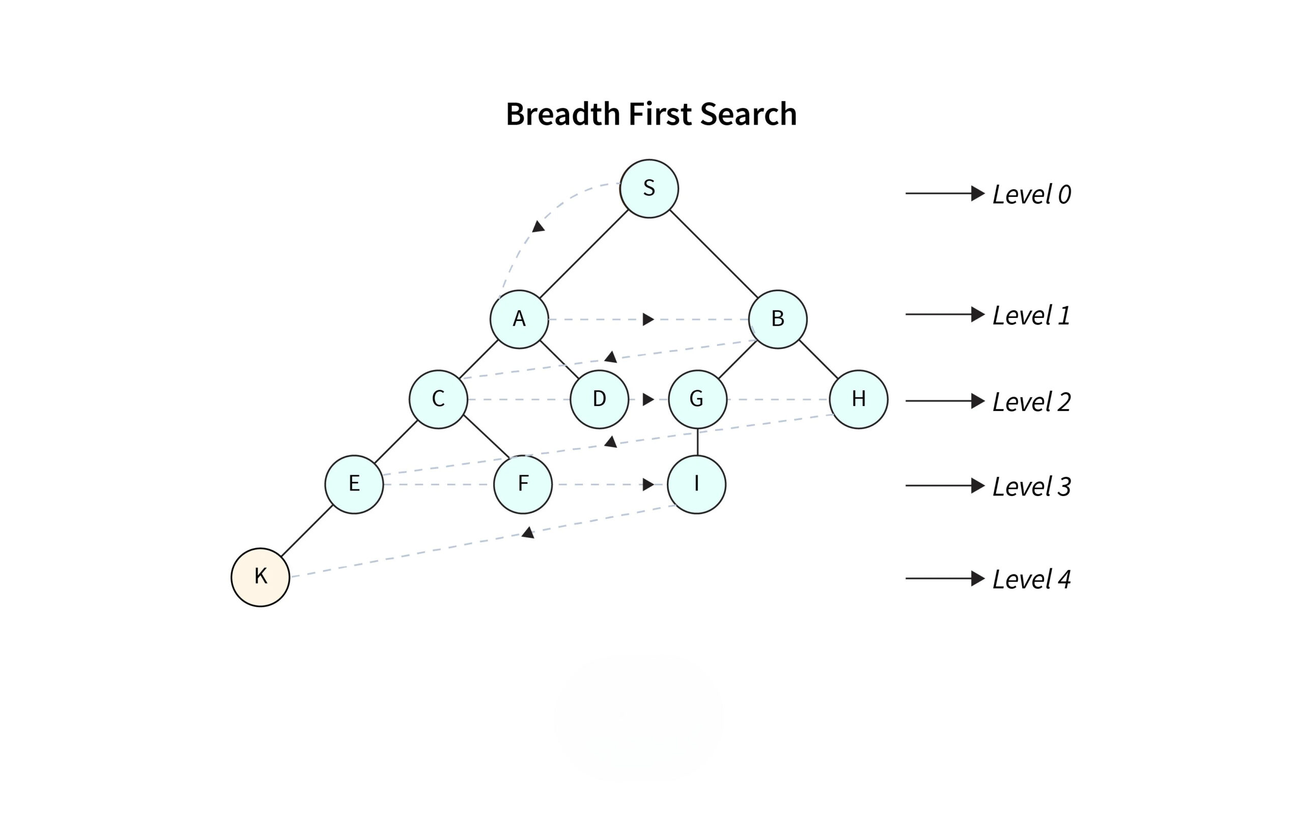
This layered approach is precisely why BFS is the perfect tool for finding the shortest path in an unweighted graph. In such a graph, the shortest path is simply the one with the fewest edges. Because BFS explores all paths of length 1 before any paths of length 2, and all paths of length 2 before any of length 3, the first time it reaches any destination node, it is guaranteed to have done so via a shortest path.

The following video provides a fantastic analogy that should resonate with your engineering background and solidifies this core concept.

2. The Algorithm Mechanics

To implement this "layer-by-layer" strategy, BFS relies on a few key data structures. Given your software engineering experience, you'll find these very familiar.

1. A Queue: To manage the order of vertices to visit. This enforces the First-In, First-Out (FIFO) discipline crucial for the level-by-level traversal. We add a vertex's neighbors to the back of the queue and always process the vertex at the front.
2. A Visited Set (or boolean array): To keep track of vertices we have already enqueued. This is essential to prevent processing the same vertex multiple times and to avoid getting stuck in infinite loops if the graph contains cycles.
3. A Parent Array/Map: To reconstruct the shortest path. For each vertex v we visit, we store the vertex u from which we discovered it. This creates a trail of "breadcrumbs" back to the source.

The following video walks through this process, showing how these data structures interact to produce a BFS traversal and find a path.

To summarize the algorithm for finding the shortest path from a source to a destination:

1. Initialization:

   • Create a queue and add the source vertex to it.
   • Create a visited array/set and mark the source as visited.
   • Create a parent array/map, and initialize all entries to a null value (e.g., -1).

2. Traversal Loop: While the queue is not empty:

   • Dequeue a vertex, let's call it current.
   • If current is the destination, the shortest path has been found. We can stop and proceed to reconstruction.
   • For each neighbor of current (this is where our adjacency list from the last lesson comes in handy):
     • If neighbor has not been visited:
       • Mark neighbor as visited.
       • Set parent[neighbor] = current.
       • Enqueue neighbor.

3. Path Reconstruction:

   • If the destination was reached, backtrack from destination to source using the parent array.
   • Start with a path list containing destination.
   • While the current node in the path is not the source, prepend its parent (parent[current_node]) to the path list.

This image provides a great all-in-one summary of the process, showing the graph, data structures, and the step-by-step trace.

3. Implementation and Complexity Analysis

Now, let's look at how this translates into code and analyze its performance.

Implementation

The following resource provides a concise, high-quality implementation that demonstrates how to maintain arrays for both distance and parent pointers.

As you saw, the implementation is a direct translation of the algorithm we described. The parent array (named p in the code) is the key to fulfilling our learning objective. By tracing it backward from the destination, we can rebuild the shortest path. If you're interested, the "Shortest path in an unweighted graph" article on GeeksforGeeks provides complete, runnable examples in several languages including Java, Python, and C++.

Complexity Analysis

Analyzing the performance of BFS is straightforward and is a direct consequence of how it operates.

• Time Complexity: $O(|V|+|E|)$

  • Every vertex is enqueued and dequeued exactly once. This gives us a cost of $O(|V|)$ for the queue operations.
  • When we process a vertex, we iterate through its adjacency list to find its neighbors. Over the entire run of the algorithm, we will look at every edge in the graph's adjacency lists once (for a directed graph) or twice (for an undirected graph, once from each endpoint). The total work done here is therefore proportional to the number of edges, $O(|E|)$.
  • Combining these, the total time complexity is $O(|V|+|E|)$.

• Space Complexity: $O(|V|)$

  • The visited array and parent array each require space proportional to the number of vertices, so $O(|V|)$.
  • The queue's maximum size depends on the graph's structure. In the worst-case scenario (a very "wide" graph, like a star graph where the source is the center), the queue might have to hold nearly all $|V|-1$ vertices at once. Therefore, the space for the queue is also $O(|V|)$.
  • The dominant factor is $|V|$, making the auxiliary space complexity $O(|V|)$.

This efficiency, combined with its ability to find shortest paths, makes BFS a fundamental and widely used algorithm.

Conclusion

In this lesson, we took a deep dive into Breadth-First Search. We started with the core principle of its layered traversal and understood why this guarantees finding the shortest path in terms of edge count.

Key Takeaways:

• BFS explores a graph in layers, starting from a source vertex and moving outward.
• It relies on a queue to maintain a FIFO order of nodes to visit, ensuring the "breadth-first" property.
• It finds the shortest path in an unweighted graph because it discovers all paths of length k before any of length k+1.
• By using a parent array to track how each vertex was discovered, we can easily reconstruct the shortest path by backtracking from the destination.
• The algorithm is highly efficient, with a time complexity of $O(|V|+|E|)$ and space complexity of $O(|V|)$, making it practical for large graphs.

Preview of the Next Lesson:

Now that you've mastered BFS, the natural next step is to explore its counterpart: Depth-First Search (DFS). While BFS explores broadly, DFS explores deeply. In the next lesson, we will see how DFS uses a different data structure (a stack, often implicitly via recursion) to traverse as far as possible down one path before backtracking. We will implement it and analyze how its different traversal strategy makes it suitable for other types of graph problems.