Hello! Welcome to the fifth module of our course. We're now shifting gears from specific algorithmic paradigms like greedy and divide-and-conquer to the vast and interconnected world of graph algorithms.
As previewed in our last lesson on Huffman coding, graphs are an incredibly powerful and versatile way to model problems—from social networks and road systems to dependencies in a software project. To work with these problems algorithmically, we first need a way to represent a graph in a computer's memory. This initial choice has profound implications for the performance and complexity of the algorithms we'll build.
Today, we'll explore the two most common methods for this task. Your learning outcome is to compare adjacency matrix and adjacency list representations for graphs and their trade-offs.
We will cover:
- The definition and structure of adjacency matrices and adjacency lists.
- How to represent both directed and undirected graphs with each method.
- A detailed analysis of their respective time and space complexities.
- The critical trade-offs that determine which representation is better suited for a given problem, focusing on the concept of sparse versus dense graphs.
This foundational lesson is crucial, as nearly every graph algorithm we study from here on—including traversals, shortest paths, and more—will be built upon one of these representations.
1. Representing a Graph
First, let's quickly formalize what a graph is. A graph is a pair , where is a set of vertices (or nodes) and is a set of edges (or connections) between pairs of vertices.
- In an undirected graph, an edge
(u, v)is the same as(v, u). - In a directed graph, an edge
(u, v)represents a one-way connection fromutov.
The challenge is how to translate this abstract structure into a concrete data structure that a program can use. The following video introduces the two primary approaches: the adjacency list and the adjacency matrix.
Graphs Representations - Adjacency Lists vs Adjacency Matrix
This video from AI Papers Academy provides a clear and well-paced introduction to both representations. It walks through the construction of each for both directed and undirected graphs.
Please watch from the beginning up to 11:16. As you watch, focus on: How an undirected graph's adjacency matrix is always symmetric. How an adjacency list is constructed for both directed (outgoing edges) and undirected graphs. The different structures: a 2D array (matrix) versus an array of lists.
2. The Adjacency Matrix
As the video explained, an adjacency matrix is a straightforward representation using a two-dimensional array.
For a graph with vertices, we create a matrix, let's call it adj. The entry adj[i][j] tells us about the edge between vertex i and vertex j.
- Structure: A
|V| x |V|grid of0s and1s. - Rule:
adj[i][j] = 1if an edge exists fromitoj; otherwise,adj[i][j] = 0. - Undirected Graphs: The matrix is symmetric (
adj[i][j] == adj[j][i]) because an edge betweeniandjimplies a connection in both directions. - Weighted Graphs: Instead of
1,adj[i][j]can store the weight of the edge. A special value (like∞or-1) is used to indicate the absence of an edge.
The primary characteristic of an adjacency matrix is its space complexity. It always requires space, regardless of how many edges the graph actually has. This makes it very simple to implement but can be inefficient for graphs with many vertices but few edges.
3. The Adjacency List
The adjacency list takes a more space-efficient, vertex-centric approach.
- Structure: An array (or a map/dictionary) of size . Each entry
adj[i]points to a linked list (or a dynamic array/vector) containing all the verticesjfor which there is an edge fromitoj. - Undirected Graphs: If there is an edge between
iandj, thenjwill appear ini's list, andiwill appear inj's list. - Weighted Graphs: The list can store pairs of
(neighbor, weight)instead of just the neighbor vertex.
The space complexity here is directly related to the number of vertices and edges. It requires space.
- for the main array of pointers/lists.
- for the total number of nodes across all linked lists. (For an undirected graph, each edge
(u,v)adds two entries, one inu's list and one inv's, for a total of entries, which is still ).
4. Analyzing the Trade-offs
Now for the central question: which representation is better? As is often the case in software engineering, the answer is, "it depends on what you need to do." The choice involves a trade-off between space usage and the time it takes to perform certain operations.
To get a detailed breakdown of these trade-offs, let's turn to a concise textual resource.
Comparison between Adjacency List and Adjacency Matrix
The following article from GeeksforGeeks provides an excellent summary table that compares the two representations across several key operations.
Please read the comparison table in the article. Focus on the time complexity (O(...)) for the following operations: Storage Space Adding an edge Removing an edge Querying (checking if an edge exists between two vertices)
Let's synthesize that information and highlight the most critical comparisons for algorithm design. Let deg(u) be the degree of vertex u (the number of edges connected to it).
| Operation | Adjacency Matrix | Adjacency List | Winner |
|---|---|---|---|
| Space | $O( | V | ^2)$ |
| Check if edge (u, v) exists | Matrix | ||
| Find all neighbors of u | $O( | V | )$ |
| Add an edge (u, v) | * | (Tie) | |
| Remove an edge (u, v) | Matrix |
*Adding an edge to an adjacency list is if you just append to the list. The complexities for adding/removing vertices are higher for both but less commonly analyzed in basic algorithm contexts.
This table reveals two key scenarios:
- If your algorithm needs to frequently check for the existence of arbitrary edges, an adjacency matrix is superior due to its query time.
- If your algorithm needs to iterate through the neighbors of vertices, an adjacency list is far more efficient. You only traverse the actual neighbors, not an entire row of
Vvertices.
This leads us to the crucial distinction between sparse and dense graphs.
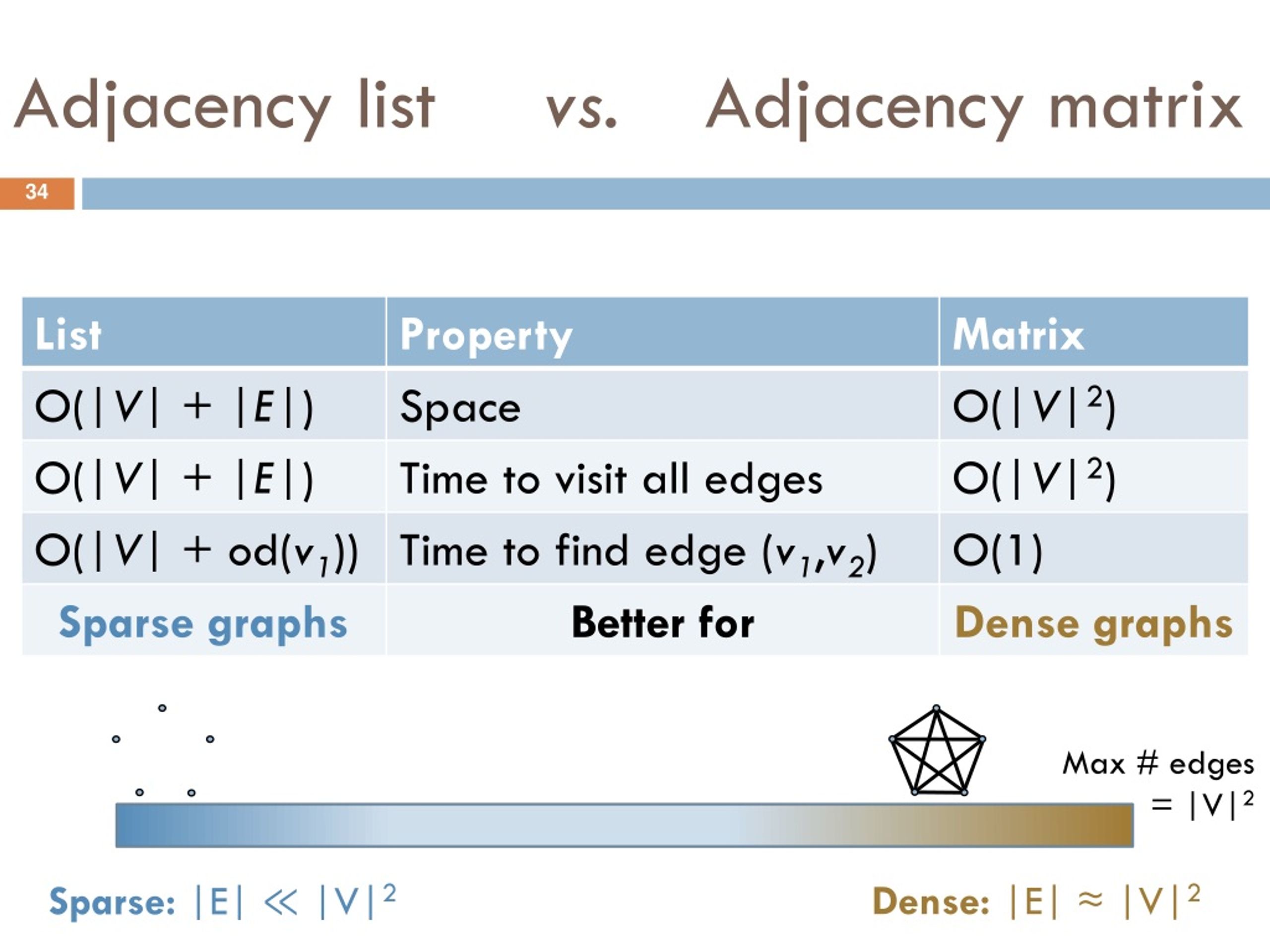
- Sparse Graph: A graph with relatively few edges. Formally, . Most real-world graphs (social networks, road networks) are sparse. For these, the space of a matrix is wasteful. The adjacency list is the clear winner.
- Dense Graph: A graph with many edges. Formally, . Here, the space complexities of both representations are asymptotically similar, so the choice may depend more on the required operations (e.g., frequent edge queries favor the matrix).
Since most graph algorithms you'll encounter (like BFS and DFS) are based on exploring a vertex's neighbors, and most problem domains involve sparse graphs, the adjacency list is the default, go-to representation for general-purpose graph programming.
Conclusion
In this lesson, we established the groundwork for our entire module on graphs. We demystified the two primary ways to store a graph in memory and, most importantly, analyzed the engineering trade-offs between them.
Key Takeaways:
- Adjacency Matrix: An space representation that offers constant-time edge existence checks. It's simple but can be very wasteful for sparse graphs.
- Adjacency List: An space representation that excels at iterating through a vertex's neighbors in time proportional to its degree.
- Sparse vs. Dense: The choice between them hinges on the density of the graph. Sparse graphs () strongly favor adjacency lists. Dense graphs () make the adjacency matrix more viable.
- For most practical applications and the upcoming algorithms we will study, the adjacency list is the preferred representation due to its space efficiency and optimized neighbor traversal.
Preview of the Next Lesson:
Now that we know how to represent a graph, we can start exploring it. In our next lesson, we will learn our first graph traversal algorithm: Breadth-First Search (BFS). We will see how BFS systematically explores a graph level by level and how it can be used to find the shortest path between two vertices in an unweighted graph. You will see firsthand why the adjacency list's ability to efficiently retrieve neighbors is so critical for this algorithm.