Dijkstra's Algorithm: Shortest Paths and Limitations

Introduction

In the previous module, we explored how to traverse graphs using BFS and DFS, focusing on connectivity and cycle detection in unweighted graphs. Now, we're taking a significant step forward by introducing weights to the edges. These weights can represent distance, time, cost, or any other metric, turning our graphs into richer models of real-world problems.

This brings us to one of the most fundamental problems in graph theory: the Single-Source Shortest Path (SSSP) problem. The goal is to find the path with the minimum total weight from a designated starting node to every other node in the graph. This has direct applications in GPS navigation (finding the fastest route), network routing (finding the most efficient data path), and many other optimization scenarios.

Today's lesson fulfills the learning outcome: Apply Dijkstra's algorithm to find single-source shortest paths and explain its limitations. We will learn how this classic greedy algorithm works, see it in action, analyze its performance, and crucially, understand the specific conditions under which it operates correctly.

1. The Core Idea of Dijkstra's Algorithm

Dijkstra's algorithm, conceived by Edsger W. Dijkstra in 1956, is a greedy algorithm. This means at each step, it makes the choice that seems best at that moment. For Dijkstra's, this means always exploring the "closest" unvisited node from the source. It systematically expands a "frontier" of visited nodes, guaranteeing that once a node is finalized, the shortest path to it has been found.

To get a high-level intuition for how this works, let's watch a short, well-animated explanation.

As you saw, the algorithm maintains a set of tentative distances to all nodes and iteratively refines them. Let's formalize the key components:

• Initialization:

  • A distances data structure (like an array or dictionary) stores the shortest distance found so far from the source to every other node. It's initialized with 0 for the source node and infinity ($\infty$) for all others.
  • A set of visited nodes is kept to avoid reprocessing.
  • A priority queue is used to efficiently store unvisited nodes and retrieve the one with the smallest tentative distance. This is the key to the algorithm's efficiency.

• The Main Loop: The algorithm repeatedly does the following until all reachable nodes are visited:

  1. Select: Extract the unvisited node u with the smallest distance from the priority queue.
  2. Visit: Mark u as visited. Its current distance is now considered final.
  3. Relax Neighbors: For each neighbor v of u, perform a "relaxation" step.

The Relaxation Step

Relaxation is the heart of the algorithm. It's the process of checking if the path to a neighbor v through the current node u is shorter than any path to v found so far.

The logic is simple:
If distances[u] + weight(u, v) < distances[v], then we have found a better path to v. We update distances[v] to this new, lower value.

2. A Step-by-Step Walkthrough

Now let's trace the algorithm on a more complex example to solidify your understanding of the selection and relaxation process.

By following this process, Dijkstra's algorithm systematically finds the shortest path from the source to all other nodes. The greedy choice of always picking the closest unvisited node works because all edge weights are non-negative. This ensures that once we select a node, we won't find a "detour" through some other unvisited node that could have resulted in a shorter path.

3. Implementation and Complexity

Given your software engineering background, seeing the algorithm in code can be very illuminating. A standard implementation uses an adjacency list to represent the graph and a min-priority queue to manage the distances.

Complexity Analysis Summary

As the article explained, the choice of data structure for finding the minimum distance node is critical:

1. Using a simple array/list:

   • In each of the $|V|$ iterations, we must scan all $|V|$ vertices to find the unvisited one with the minimum distance.
   • This leads to a time complexity of $O(|V{|}^2)$. This is acceptable for dense graphs (where $|E|$ is close to $|V{|}^2$), but inefficient for sparse graphs (where $|E|$ is closer to $|V|$).

2. Using a Binary Heap (Priority Queue):

   • Building the initial heap takes $O(|V|)$.
   • The main loop runs $|V|$ times, and each extract-min operation from the heap takes $O(\log |V|)$ time.
   • Every edge is relaxed at most once. Each relaxation might lead to a decrease-key operation (by pushing a new, smaller-distance entry), which takes $O(\log |V|)$ time. In the worst case, this happens for all $|E|$ edges.
   • This gives a total time complexity of $O(|V|\log |V|+|E|\log |V|)$, often simplified to $O((|V|+|E|)\log |V|)$ or just $O(|E|\log |V|)$ for connected graphs. This is the standard and much more efficient approach for sparse graphs.

The space complexity is $O(|V|+|E|)$ to store the graph, distances, and the priority queue.

4. The Critical Limitation: Negative Edge Weights

Dijkstra's greedy strategy hinges on one crucial assumption: all edge weights are non-negative. If a graph contains even one negative edge, the algorithm can produce incorrect results.

The reason is that the algorithm's guarantee is broken. When Dijkstra's finalizes the distance to a node u, it assumes there's no shorter path to be found. However, a path through a later-visited node v that involves a negative edge might reveal a "shortcut" back to u or one of its neighbors, a possibility the algorithm doesn't account for.

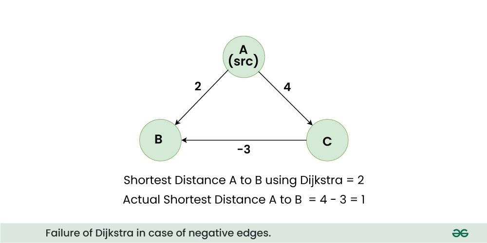
This next video segment demonstrates this failure case very clearly.

This limitation is not a minor detail; it is the single most important constraint to remember when deciding whether to use Dijkstra's algorithm.

Conclusion

In this lesson, we have taken a deep dive into one of the cornerstones of graph algorithms. You can now apply Dijkstra's algorithm and, just as importantly, know when not to apply it.

Key Takeaways:

• Dijkstra's algorithm solves the single-source shortest path problem for graphs with non-negative edge weights.
• It is a greedy algorithm that works by maintaining a set of tentative distances and always visiting the closest unvisited node.
• The core operation is relaxation, where paths to neighbors are updated if a shorter route is found.
• An efficient implementation uses a priority queue (min-heap) to achieve a time complexity of $O((|V|+|E|)\log |V|)$.
• The primary limitation of Dijkstra's algorithm is its failure to produce correct results on graphs containing negative edge weights.

Preview of the Next Lesson:
So, what do we do when our graph does have negative edge weights, which can happen in many real-world models (e.g., representing financial gains and losses)? In our next lesson, we will tackle this exact problem by learning the Bellman-Ford algorithm. It is slower than Dijkstra's, but it is more robust, capable of handling negative weights, and can even be used to detect the presence of "negative cycles."