Bellman-Ford: Handling Negative Edge Weights and Cycles

Introduction

In our last lesson, we explored Dijkstra's algorithm, a fast and efficient method for finding the shortest paths from a single source. However, we also discovered its crucial limitation: it fails when a graph contains edges with negative weights. The greedy approach of finalizing the "closest" node breaks down when a future path could offer a "shortcut" via a negative-cost edge.

This lesson directly addresses that limitation, fulfilling the learning outcome: Apply the Bellman-Ford algorithm for graphs with negative edge weights and to detect negative cycles.

The Bellman-Ford algorithm is slower than Dijkstra's, but it's more robust. It can handle graphs with negative edge weights, and it has a built-in mechanism to detect the presence of negative-weight cycles—a situation where shortest paths can become undefined (infinitely small). This makes it an indispensable tool for a wider range of graph problems, particularly in areas like finance where negative costs or losses are common.

1. The Core Idea: Systematic Relaxation

Unlike Dijkstra's greedy approach, Bellman-Ford is fundamentally based on dynamic programming. It solves the problem by systematically building up the solution. The core idea is that the shortest path from a source s to any vertex v can have at most $|V|-1$ edges (where $|V|$ is the number of vertices), assuming no negative cycles exist. If a path had more edges, it would have to contain a cycle, which wouldn't be optimal unless the cycle had a negative weight.

Based on this insight, the Bellman-Ford algorithm works by repeatedly relaxing every edge in the graph. It performs this relaxation process for $|V|-1$ passes.

• After 1 pass, it has found all shortest paths that are at most 1 edge long.
• After 2 passes, it has found all shortest paths that are at most 2 edges long.
• ...
• After $k$ passes, it has found all shortest paths that are at most $k$ edges long.

Therefore, after $|V|-1$ passes, the algorithm is guaranteed to have found all shortest simple paths.

To understand this foundational concept and how it differs from Dijkstra's, let's start with a clear overview.

The process described in the video—initializing distances and then repeatedly relaxing all edges—is the heart of the algorithm. Let's look at the formal steps.

2. A Step-by-Step Walkthrough

Now that you have the high-level idea and the formal structure, let's walk through a complete example. Seeing the distance values update with each pass is the best way to understand how the algorithm converges to the correct answer.

The following image provides a static, step-by-step trace of the algorithm.

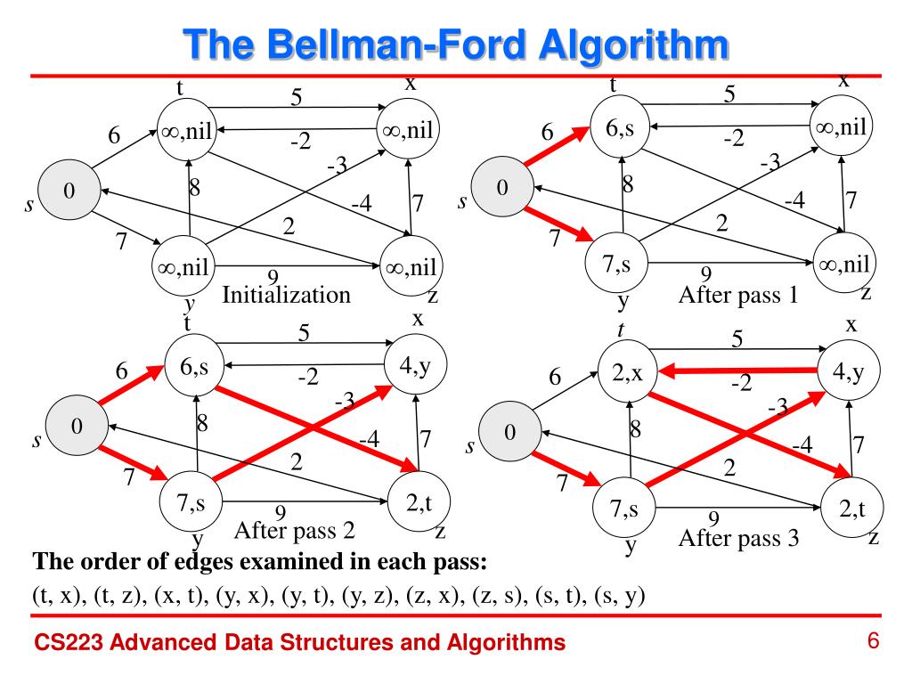
To see this process in a more dynamic fashion, let's return to the WilliamFiset video.

3. Detecting Negative Cycles

One of Bellman-Ford's most powerful features is its ability to detect negative-weight cycles. The logic is elegant:

• We've established that any shortest path in a graph with no negative cycles can have at most $|V|-1$ edges.
• After $|V|-1$ passes, the algorithm has found these paths.
• What happens if we run the algorithm for one more pass (the $|V|$-th pass)? If any distance value can still be improved, it means we've found a shorter path that must involve at least $|V|$ edges. A path with $|V|$ edges through $|V|$ vertices must contain a cycle.
• Since the path's weight was reduced by traversing this cycle, the cycle's total weight must be negative.

So, the detection method is simple: After the main $|V|-1$ passes, perform one final pass. If any edge can still be relaxed, a negative cycle exists.

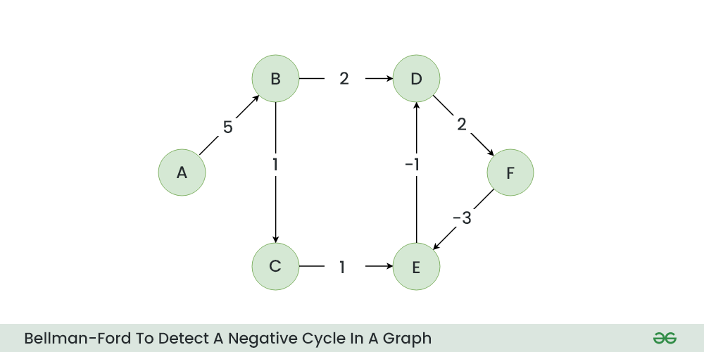
The following video demonstrates this detection process.

Once a negative cycle is detected, the shortest paths to any nodes that are part of the cycle or are reachable from it are undefined (or can be considered negative infinity), as you can traverse the cycle endlessly to reduce the path cost.

4. Proof of Correctness and Complexity

Your preference for understanding the "why" behind algorithms is key here. The proof of Bellman-Ford's correctness is a classic inductive argument that's quite intuitive.

Complexity Analysis

The complexity of Bellman-Ford is straightforward to analyze, which your software engineering background will make immediately apparent.

• The algorithm consists of a main loop that runs $|V|-1$ times (for the path finding) plus potentially one more time (for cycle detection). Let's say this is $O(|V|)$ passes.
• Inside this loop, the algorithm iterates through all $|E|$ edges and performs a constant-time relaxation operation for each.

Therefore, the total time complexity is $O(|V|\cdot |E|)$.

• In a sparse graph (where $|E|$ is close to $|V|$), the complexity is about $O(|V{|}^2)$.
• In a dense graph (where $|E|$ is close to $|V{|}^2$), the complexity becomes $O(|V{|}^3)$.

This is significantly slower than Dijkstra's $O((|V|+|E|)\log |V|)$, which is why Dijkstra's is preferred whenever you can guarantee non-negative edge weights.

The space complexity is $O(|V|)$ to store the distances and predecessors.

Conclusion

In this lesson, we've added a powerful and robust tool to our algorithmic toolbox. While slower than Dijkstra's, Bellman-Ford's ability to handle negative weights and detect negative cycles makes it applicable to a much broader class of problems.

Key Takeaways:

• The Bellman-Ford algorithm solves the single-source shortest path problem for graphs that may contain negative edge weights.
• It works by relaxing all edges in the graph for $|V|-1$ passes.
• It can detect a negative-weight cycle by running one additional pass ($V$-th pass); if any edge can still be relaxed, a negative cycle reachable from the source exists.
• The time complexity is $O(|V|\cdot |E|)$, making it slower than Dijkstra's but more general.

Preview of the Next Lesson:
We will now shift our focus from finding shortest paths to another fundamental graph problem: finding a Minimum Spanning Tree (MST). An MST is a subset of edges that connects all vertices together with the minimum possible total edge weight, without forming any cycles. To tackle this, we'll first need to learn about a specialized data structure perfect for detecting cycles: the Union-Find data structure. We'll explore its implementation with optimizations like path compression and union by rank.