PCA: Reducing Dimensions with Maximum Variance

Introduction

In our last lesson, we established why dimensionality reduction is so critical. You learned that high-dimensional data is difficult to visualize and can lead to the "curse of dimensionality," which hurts model performance through issues like data sparsity and overfitting.

Today, we move from the why to the how. This lesson focuses on explaining one of the most fundamental and widely used dimensionality reduction techniques: Principal Component Analysis (PCA). Our goal is to understand how PCA works its magic by finding and prioritizing the directions in your data that contain the most information. In line with your preference for a theory-first approach, we will build a solid conceptual and mathematical foundation that will prepare you for implementing PCA in Python in our next session.

Part 1: The Core Idea - Finding the Best "View" of Your Data

Imagine your data is a massive, complex cloud of points in a high-dimensional space. If you were to look at this cloud from a random angle, you might not see much structure—it could look like a formless blob. However, from another angle, you might see the data is stretched out, revealing its most important features.

PCA is an algorithm that mathematically finds the "best" viewing angles for your data. In PCA, the "best" view is the one that shows the most variation or spread in the data. The core principle is that variance equals information. A feature that doesn't vary much tells us little, but a feature with high variance is rich with information.

Let's start by visualizing this central idea.

PCA: Conceptual Algorithm - Maximum Variance — This image shows a scatter plot of data. The goal of PCA is to find the line (the red principal component) where the projection of the data points results in the maximum possible spread, or variance.

To build on this, we'll watch a segment of a video that provides a brilliant step-by-step intuition for how PCA finds this line of maximum variance.

StatQuest: Principal Component Analysis (PCA), Step-by-Step

The video 'StatQuest: Principal Component Analysis (PCA), Step-by-Step' provides an exceptionally clear, visual explanation of PCA's mechanics. We'll focus on how it identifies the first and most important component.

Watch the segment from 03:32 to 10:20. Pay close attention to how the data is first centered, and then a line is rotated until it finds the orientation that maximizes the sum of the squared distances of the projected points from the origin. This is the key to understanding 'maximum variance'.

As the video explained, the first Principal Component (PC1) is the line that best represents the data's primary direction of spread. It's the axis that captures the most variance.

Part 2: From One Component to a New Coordinate System

Finding PC1 is a great start, but we've only captured one dimension of our data. What about the rest of the information?

PCA builds a new coordinate system by finding subsequent components. After identifying PC1, it looks for the next direction of maximum variance, with one crucial constraint: the new direction must be orthogonal (at a right angle) to PC1. This ensures that the new component, PC2, is capturing new, uncorrelated information. This process continues, with each new principal component being orthogonal to all previous ones and capturing the maximum remaining variance.

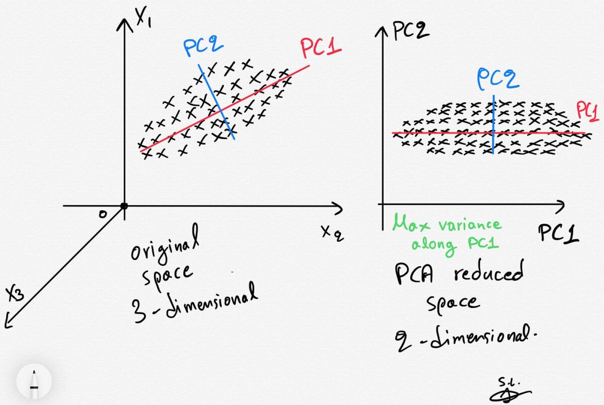
PCA Dimensionality Reduction Illustration — This image illustrates the process. In a 3D dataset (left), PCA first finds PC1 (red), the direction of maximum variance. It then finds PC2 (blue), which is orthogonal to PC1 and captures the most remaining variance. By projecting the data onto the 2D plane defined by PC1 and PC2, we get a lower-dimensional representation (right) that preserves most of the original structure.

This new set of axes (PC1, PC2, PC3, ...) forms a new coordinate system that is perfectly aligned with the variance in your data.

The Mathematical Connection: Eigenvectors and Eigenvalues

This is where your linear algebra background becomes relevant. The process of finding these special directions of maximum variance is mathematically equivalent to finding the eigenvectors of the data's covariance matrix.

Let's connect these concepts by reading a clear explanation.

Principal Component Analysis (PCA): Complete Guide

The article 'Principal Component Analysis (PCA): Complete Guide' from TensorTonic has an excellent section explaining the intuition and the underlying math involving the covariance matrix.

First, read the section 'The Core Intuition' to solidify the 'pancake' analogy. Then, carefully read 'The Covariance Matrix'. Focus on the final paragraph under that heading: it explicitly states that the eigenvectors of the covariance matrix are the principal components, and the eigenvalues tell us how much variance each one captures.

To summarize the critical insight from the reading:

Principal Components are Eigenvectors: The directions of maximum variance (PC1, PC2, etc.) are the eigenvectors of the covariance matrix of your data.
Variance is an Eigenvalue: The amount of variance captured by each principal component is given by its corresponding eigenvalue.

Therefore, to find the most important principal component (PC1), we simply find the eigenvector of the covariance matrix with the largest eigenvalue. PC2 is the eigenvector with the second-largest eigenvalue, and so on.

Part 3: The PCA Algorithm and Measuring Variance

Let's formalize this into a step-by-step process. While the underlying math can be complex, the algorithm itself is quite logical. We can also explore the mathematical proof that maximizing variance leads directly to this eigenvalue problem.

Principal Component Analysis Part 1: The Different Formulations.

This article, 'Principal Component Analysis Part 1: The Different Formulations', provides a rigorous but clear mathematical derivation. We'll focus on the 'Maximum Variance Formulation' which proves why eigenvectors are the solution.

Read the section 'PCA: Maximum Variance Formulation'. You don't need to memorize every equation, but follow the logic: it sets up an optimization problem to maximize variance (Eq. 4) under a constraint, and using Lagrange multipliers, it shows the solution (Eq. 8) is the eigenvalue equation. This directly proves that the direction w that maximizes variance must be an eigenvector of the covariance matrix S.

This derivation solidifies the "theory-first" understanding of PCA. The algorithm, then, is a practical application of this proof.

The Algorithm at a High Level

Standardize the Data: PCA is sensitive to the scale of your features. If one feature (e.g., income in dollars) has a much larger range than another (e.g., age in years), it will dominate the variance calculation. Therefore, the first step is to standardize each feature to have a mean of 0 and a standard deviation of 1.
Compute the Covariance Matrix: Calculate the covariance matrix for the standardized data. This d x d matrix (where d is the number of dimensions/features) describes how every feature varies with every other feature.
Perform Eigendecomposition: Compute the eigenvectors and eigenvalues of the covariance matrix.
Select Principal Components: Sort the eigenvectors in descending order based on their corresponding eigenvalues. The eigenvector with the largest eigenvalue is PC1, the second is PC2, and so on. You then choose the top k eigenvectors to be your new dimensions.
Project the Data: Transform the original, standardized data into the new k-dimensional space by projecting it onto the selected principal components.

How much variance is captured?

The explained variance ratio for each principal component tells us the proportion of the dataset's total variance that it accounts for. It's calculated as:

Explained Variance Ratio of PC_{i} = \frac{λ _{i}}{\sum _{j = 1}^{d} λ _{j}}

Where $λ_{i}$ is the eigenvalue of the i-th principal component and the denominator is the sum of all eigenvalues. By looking at the cumulative sum of these ratios, we can decide how many components to keep to retain a desired percentage (e.g., 95%) of the total information.

Conclusion

In this lesson, we dissected the mechanics of Principal Component Analysis. You've moved beyond knowing why we need to reduce dimensions to understanding how PCA achieves this by intelligently rotating our dataset to find new axes based on maximum variance.

Key Takeaways:

PCA reduces dimensionality by finding a new set of orthogonal axes, called principal components, that align with the directions of maximum variance in the data.
The first principal component (PC1) captures the most variance, PC2 captures the second most (and is orthogonal to PC1), and so on.
Mathematically, the principal components are the eigenvectors of the data's covariance matrix.
The eigenvalues corresponding to these eigenvectors represent the amount of variance captured by each principal component.
The explained variance ratio tells us what percentage of total information each component holds, helping us decide how many components to keep.

Preview of the Next Lesson:
With this theoretical framework firmly in place, you are ready for the practical application. In the next lesson, you will apply PCA to a dataset using scikit-learn. We will take these concepts—standardization, fitting, and transformation—and execute them with just a few lines of Python code to reduce the dimensionality of a real dataset and visualize the result.

Recommended resources