Understanding Overfitting, Underfitting, and the Bias-Variance Tradeoff

1. The Twin Problems: Overfitting and Underfitting

When we train a machine learning model, we are looking for a "good fit." We want a model that captures the true underlying patterns in the data but ignores the random noise. Two things can go wrong: the model can be too simple (underfitting) or too complex (overfitting).

Let's start with a quick visual intuition for these two problems.

Now, let's formalize these definitions and look at some real-world examples.

From the video and reading, we can summarize the key characteristics:

• Underfitting:

  • Symptom: The model performs poorly on both the training data and the test data.
  • Cause: The model is too simple to capture the underlying structure of the data. It fails to learn.
  • Example: Using a simple linear model to predict house prices when the relationship also depends on complex factors like location and age.

• Overfitting:

  • Symptom: The model performs exceptionally well on the training data but poorly on the test data.
  • Cause: The model is too complex. It has effectively "memorized" the training data, including its random noise, and has not learned the general pattern. It fails to generalize.
  • Example: A medical diagnosis model that memorizes artifacts in the training images instead of learning the general features of a disease.

2. The Cause: Bias and Variance

Overfitting and underfitting are symptoms of a deeper issue related to two types of error in machine learning: bias and variance. Understanding these two concepts is the key to diagnosing model performance.

A great way to build intuition is with a target-shooting analogy. Imagine you are an archer and your goal is to hit the bullseye (the true value).

Let's break this down:

• High Bias, Low Variance: Your shots are tightly clustered but far from the bullseye. You are consistently wrong. This is like an underfit model, which makes overly simple assumptions and consistently misses the true relationship.
• Low Bias, High Variance: Your shots are scattered all around the bullseye. On average, you're centered on the target, but any single shot could be far off. You are inconsistently right. This is like an overfit model, which is so sensitive to the training data that it would produce wildly different predictions if trained on a slightly different dataset.
• High Bias, High Variance: Your shots are scattered and far from the bullseye. A worst-case scenario.
• Low Bias, Low Variance: Your shots are tightly clustered around the bullseye. This is the goal: a model that is both accurate and reliable.

Now, let's see how this plays out with a machine learning model.

To summarize the connection:

• A model with high bias pays very little attention to the training data and makes overly simple assumptions. This leads to underfitting.
• A model with high variance pays too much attention to the training data, fitting even the random noise. This leads to overfitting.

3. The Bias-Variance Tradeoff

You might now be thinking: "Great, let's just build a model with low bias and low variance!" Unfortunately, these two errors have an inverse relationship. Decreasing one tends to increase the other. This is called the bias-variance tradeoff.

The key to managing this tradeoff is adjusting model complexity.

• A very simple model (like linear regression) has high bias and low variance.
• A very complex model (like a deep decision tree or a high-degree polynomial) has low bias and high variance.

Your task as a machine learning practitioner is to find the "sweet spot" in the middle.

The relationship between model complexity, bias, variance, and total error can be visualized perfectly with the following graph. This is one of the most important conceptual diagrams in machine learning.

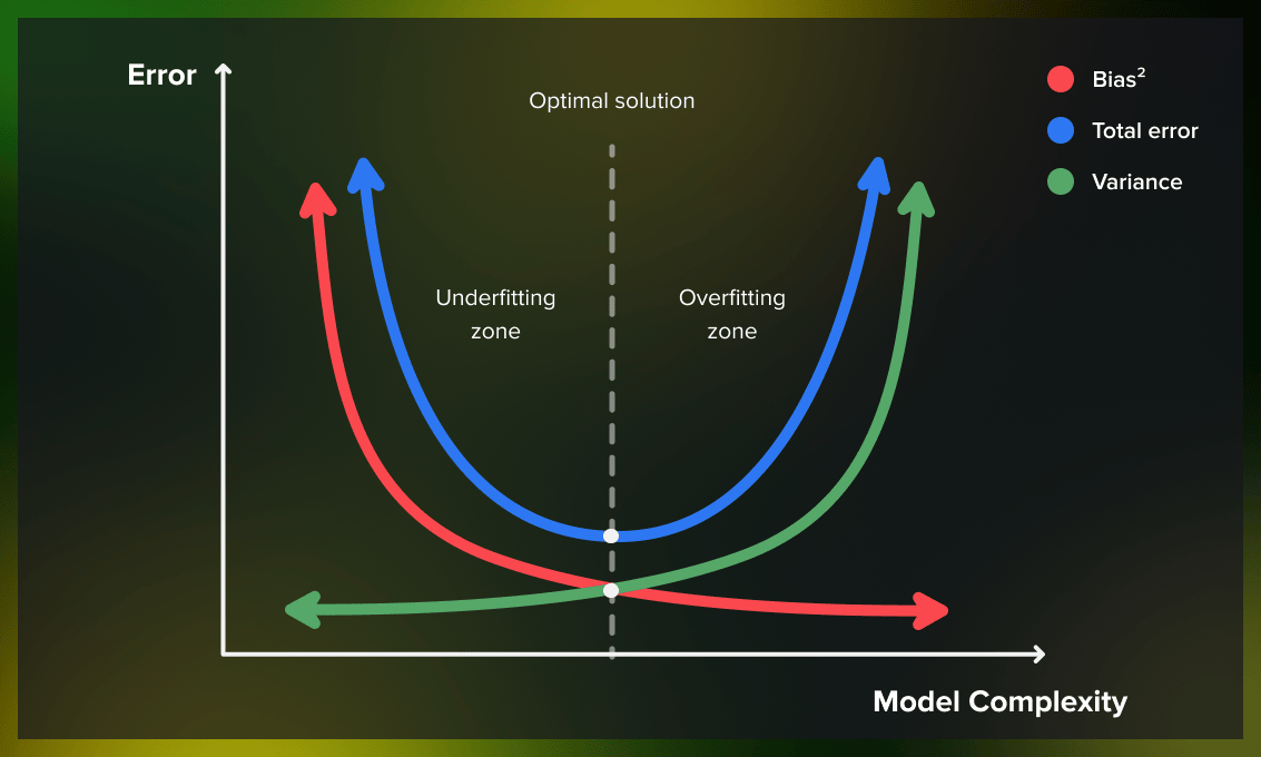
Notice the blue line for total error. Our goal is to find the level of model complexity that sits at the very bottom of that "U" shape. This is the model that generalizes best to new data.

A Glimpse into the Theory

For a deeper theoretical understanding, it's useful to know that the total expected error of a model can be mathematically decomposed. For any given data point, the expected error of your model's prediction is:

• Bias²: The error introduced by the model's simplifying assumptions.
• Variance: The error from the model's sensitivity to the specific training data it saw.
• Irreducible Error: A baseline level of error that comes from the natural randomness or noise in the data itself. This error cannot be eliminated, no matter how good the model is.

This decomposition confirms that to minimize total error, we must find an optimal balance between bias and variance.

Conclusion

In this lesson, you have explored the fundamental challenge of building models that generalize well. You've moved beyond just measuring performance and can now diagnose why a model might be failing.

Key Takeaways:

• Underfitting occurs when a model is too simple (high bias), failing to capture the underlying patterns in the data. It performs poorly on both training and test sets.
• Overfitting occurs when a model is too complex (high variance), memorizing the training data, including its noise. It performs well on the training set but poorly on the test set.
• The Bias-Variance Tradeoff is the central conflict in supervised learning: increasing model complexity reduces bias but increases variance, and vice versa.
• The goal is to find the optimal model complexity that minimizes the total error, striking a balance between underfitting and overfitting.

Preview of the Next Lesson:
We've discussed model error conceptually (high vs. low). But how do we measure it precisely? In the next lesson, you will learn to select and apply appropriate evaluation metrics for a given problem (e.g., accuracy, Mean Squared Error). These metrics are the tools you'll use to calculate the training and test errors that reveal whether your model is underfit, overfit, or just right.