Backpropagation and Gradient Descent

Introduction

In our last lesson, we traced the path of information flowing forward through a neural network to generate a prediction. We saw how an input, like the pixels of an image, is transformed layer by layer until the network produces an output. But what happens when that output is wrong? A network with random weights will initially produce random, useless predictions. The essence of "learning" is correcting these errors.

This brings us to the core of how neural networks learn: an elegant and powerful algorithm called backpropagation. Today's learning outcome is to explain the concept of backpropagation and its role in calculating gradients for learning.

We know from our earlier look at gradient descent that to minimize a cost function, we need to calculate its gradient—the direction of steepest ascent. Backpropagation is the algorithm that computes this gradient for a neural network's cost function, not just with respect to one or two variables, but with respect to the thousands or even millions of weights and biases in the network. It's the mechanism that tells us exactly how to "nudge" each parameter to improve the network's performance.

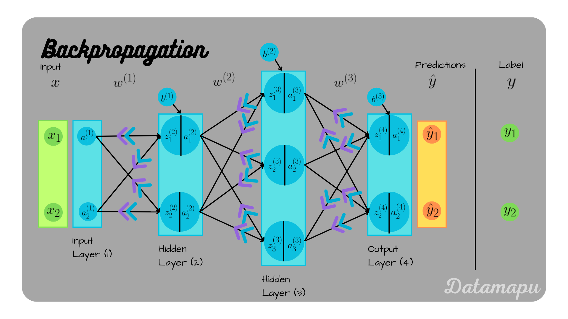
Backpropagation in a Neural Network — This diagram illustrates the two-way flow in a neural network during training. The **Forward Pass** generates a prediction, and the **Backward Pass** (backpropagation) propagates the error signal backward to calculate the gradients needed for learning.

The Core Intuition: Assigning Blame

Before diving into the mathematics, let's build an intuition for what backpropagation is trying to achieve. Imagine the network makes a mistake—it sees an image of a "2" but outputs a high activation for "8". The cost function tells us how big the error is. Backpropagation's job is to figure out who is to blame for that error and how to correct it.

It does this by propagating the error signal backward from the output layer.

At the output layer: It's easy to see which neurons are wrong. The neuron for "8" should have been less active, and the one for "2" should have been more active. We have a clear "desired change".
Propagating to the hidden layers: The algorithm then looks at the connections leading to the erroneous output neurons. A connection (weight) is considered more "responsible" if it was connected to a highly active neuron in the previous layer. The intuition is that this connection had a larger influence on the final, incorrect output.
Recursive process: This process repeats, layer by layer, moving backward. The desired changes for one layer become the basis for calculating the desired changes in the preceding layer. Each weight and bias in the network receives a "blame signal"—its gradient—proportional to its contribution to the total error.

This video from 3Blue1Brown provides a superb visualization of this intuitive process.

Backpropagation, intuitively | Deep Learning Chapter 3

Let's watch 'Backpropagation, intuitively' by 3Blue1Brown to see this concept in action. This video masterfully explains the idea without getting bogged down in formulas initially.

Please watch from the beginning to 08:28. Focus on these key ideas: How the error at the output layer creates a set of 'desired nudges' for the final activations. How these nudges are used to determine the desired changes for the weights, biases, and activations of the previous layer. The principle of proportionality: why are changes to some weights more impactful than others? Pay attention to the discussion of connections from brighter neurons having a bigger effect.

As the video explains, backpropagation is essentially a systematic way of assigning credit or blame for the final error, allowing us to adjust the parameters in the most effective way to reduce that error. The phrase "neurons that fire together, wire together" loosely captures this: connections that contribute most to a desired (or undesired) outcome are the ones that get modified the most.

The Mechanism: The Chain Rule in a Computational Graph

The mathematical engine that drives this backward propagation of error is the chain rule from calculus. A neural network, no matter how complex, is just a giant composite function. The output of the first layer is the input to the second, whose output is the input to the third, and so on.

To calculate the derivative of the final loss with respect to a weight deep inside the network (e.g., in the first layer), we need the chain rule to link all the intermediate functions together.

A powerful way to visualize this is to think of the network as a computational graph, where each node (or "gate") performs a simple operation.

Backpropagation - CS231n

The Stanford CS231n course notes provide one of the clearest explanations of backpropagation as a local process on a computational graph. This perspective is key to understanding how it can be implemented efficiently.

Read the sections titled 'Compound expressions with chain rule' and 'Intuitive understanding of backpropagation'. Focus on: How the example f(x,y,z) = (x + y) * z is broken down into simpler parts (q = x + y, f = q * z). How the chain rule (df/dx = df/dq * dq/dx) multiplies the 'local' gradient (dq/dx) by the gradient flowing back from the rest of the circuit (df/dq). The key insight: Backpropagation is a 'beautifully local process.' Each gate only needs to know its local gradient and the gradient from the gate ahead of it.

This "local process" is what makes backpropagation so powerful and efficient. Each part of the network can compute its own small piece of the gradient, and the chain rule provides the recipe for combining them correctly.

To make this perfectly concrete, let's examine the simplest possible case: a network with a single input, a single output, and just one weight.

0:03 / 9:21The Absolutely Simplest Neural Network Backpropagation Example

This video, 'The Absolutely Simplest Neural Network Backpropagation Example' by Mikael Laine, walks through the calculus for a tiny network. It will show you exactly how the chain rule is applied.

Watch from the beginning to 08:15. You will see how to calculate the gradient of the error with respect to the single weight W. Pay close attention to: The error function: Error = (a - y)^2 (where a is the network's output and y is the target). The goal: We want to find d(Error)/dW. The chain rule application: d(Error)/dW = d(Error)/da * da/dW. The video clearly calculates each part and multiplies them together.

This simple example reveals the entire secret. Backpropagation is nothing more than repeated application of this principle, chained backward through all the layers, weights, and activation functions of the network.

The Full Algorithm: The Backward Pass

Now we can put all the pieces together and look at the full backward pass for a multi-layer network. During the forward pass, we cache the pre-activation values ( $z^{[ℓ]}$ ) and activation values ( $a^{[ℓ]}$ ) for each layer. We need them for the backward pass.

The process starts at the end and moves backward from layer $L$ to layer 1.

Forward and Backward Pass in a Neural Network — This diagram shows the equations for both the forward and backward passes. Trace the 'Backward Pass' section. Notice how the calculation of the gradient for a layer (e.g., ∂L/∂W1) depends on the gradient calculated for the next layer (e.g., ∂L/∂z2).

Let's break down the flow shown in the diagram above:

Compute the gradient at the output: The first step is to calculate the derivative of the Loss $L$ with respect to the final layer's activation, $\partial L / \partial a_{2}$ . This depends on the specific loss function we chose (e.g., Mean Squared Error).
Propagate through the last activation function: Using the chain rule, we find the gradient with respect to the pre-activation $z_{2}$ :
$\frac{\partial L}{\partial z _{2}} = \frac{\partial L}{\partial a _{2}} \circ ϕ^{'} (z_{2})$
(The $\circ$ denotes element-wise multiplication).
Calculate gradients for the last layer's parameters: Now that we have $\partial L / \partial z_{2}$ , we can find the gradients for the weights $W_{2}$ and biases $b_{2}$ of the final layer. The derivative of $z_{2} = W_{2} a_{1} + b_{2}$ with respect to $W_{2}$ is just $a_{1}$ . So, by the chain rule:
$\frac{\partial L}{\partial W _{2}} = \frac{\partial L}{\partial z _{2}} (a_{1})^{T}$
Propagate the gradient to the previous layer: We continue moving backward, calculating the gradient with respect to the previous layer's activations, $a_{1}$ :
$\frac{\partial L}{\partial a _{1}} = (W_{2})^{T} \frac{\partial L}{\partial z _{2}}$
Repeat: Now we have $\partial L / \partial a_{1}$ . We can repeat steps 2-4 for layer 1: calculate $\partial L / \partial z_{1}$ , then $\partial L / \partial W_{1}$ and $\partial L / \partial b_{1}$ .

This process continues until we have the gradients for all parameters in the network. The set of all these gradients, $\nabla C$ , is exactly what we need for our gradient descent update step:
$W^{[ℓ]} := W^{[ℓ]} - α \frac{\partial L}{\partial W ^{[ℓ]}}$

A Note on Efficiency: Reverse-Mode Autodifferentiation

This specific method of applying the chain rule, from output to input, is also known as reverse-mode automatic differentiation. For training neural networks, where we have many input parameters (weights) and a single output (the scalar loss value), this mode is vastly more efficient than the "forward-mode" alternative. It allows us to compute all gradients with roughly the same computational cost as the forward pass itself, a remarkable and crucial property that makes training deep networks feasible.

Conclusion

In this lesson, we've pulled back the curtain on the "magic" of how neural networks learn. We've seen that backpropagation is not an opaque or mystical process, but a clever and efficient application of a fundamental concept from calculus: the chain rule.

Key Takeaways:

Backpropagation is the algorithm used to efficiently compute the gradient of the loss function with respect to every weight and bias in a neural network.
Intuitively, it works by propagating an "error signal" backward through the network, assigning "blame" to the parameters that contributed most to the final error.
Mathematically, it is an application of the chain rule on the network's computational graph. It is a "local" process, where each component only needs its local gradient and the gradient from the component in front of it.
The gradients computed by backpropagation are then fed into an optimization algorithm like gradient descent to update the network's parameters and reduce the loss.
This process is efficient because it caches values from the forward pass and uses reverse-mode autodifferentiation, which is ideal for the many-to-one structure of network training (many parameters, one loss value).

Preview of the Next Lesson:
We have now covered the complete theoretical cycle of training: a forward pass to make a prediction, a loss function to measure the error, and a backward pass (backpropagation) to calculate the gradients for learning.

Manually implementing this for every network would be incredibly tedious and error-prone. In the next lesson, we will see how modern deep learning frameworks like Keras and TensorFlow automate this entire process. You will learn to build and compile a sequential model, and when you call model.fit(), you will now understand the immense computational dance of forward and backward passes that is happening under the hood to make your network learn.