Introduction to Matplotlib for Basic Plotting

1. The Anatomy of a Matplotlib Plot

Before we start plotting, it's helpful to understand the main components of a Matplotlib visualization. This theory-first approach will make the practical code much easier to understand.

To summarize the key concepts:

• Figure: The top-level container for everything. You can think of it as the canvas.
• Axes: An individual plot within the Figure. A Figure can have one or more Axes. This is where you'll use functions like .plot() or .hist() to draw your data.
• Axis: These are the number-line-like objects that control the plot's data limits, ticks, and tick labels for the x and y dimensions. Note the difference in spelling: Axes (plural of Axis, the object) vs. Axis (the x or y dimension).

There are two primary ways to use Matplotlib:

1. Pyplot Style: You use functions from the matplotlib.pyplot module (aliased as plt) to implicitly act on the "current" Figure and Axes. It's quick for simple plots.
2. Object-Oriented (OO) Style: You explicitly create Figure and Axes objects (fig, ax = plt.subplots()) and then call methods directly on them (e.g., ax.plot()). This style gives you more control and is recommended for more complex plots and reusable code.

We will primarily use the OO style in our examples as it's a more robust practice for building larger applications.

2. Line Plots: Visualizing Trends

A line plot is the most basic and common type of plot. It's ideal for visualizing a trend in data over a continuous interval or sequence, such as changes over time.

Let's start with a video that demonstrates how to create your first plot.

Here is a summary of the steps using the object-oriented style, which you'll find is very similar:

import matplotlib.pyplot as plt
import numpy as np




# 1. Prepare data
x = np.linspace(0, 10, 100) # 100 points from 0 to 10
y = np.sin(x)




# 2. Create Figure and Axes
fig, ax = plt.subplots()




# 3. Plot the data on the Axes
ax.plot(x, y)




# 4. Customize the plot
ax.set_title('Sine Wave')
ax.set_xlabel('x-axis')
ax.set_ylabel('sin(x)')
ax.grid(True) # Add a grid for better readability




# 5. Show the plot
plt.show()

3. Scatter Plots: Showing Relationships

While a line plot connects points in a sequence, a scatter plot simply places a marker for each data point. This is perfect for visualizing the relationship between two separate numerical variables. For example, does a car's weight affect its mileage? A scatter plot can help you see the correlation.

A more direct way is to use the ax.scatter() method. Let's see this in action.

Here is a code example using ax.scatter():

# 1. Prepare data
# Generate some random data for demonstration
np.random.seed(42) # for reproducibility
x_data = np.random.rand(50) * 100 # 50 random numbers
y_data = x_data + (np.random.rand(50) - 0.5) * 50




# 2. Create Figure and Axes
fig, ax = plt.subplots()




# 3. Plot the data
ax.scatter(x_data, y_data, alpha=0.7) # alpha adds transparency




# 4. Customize
ax.set_title('Relationship between X and Y')
ax.set_xlabel('X Value')
ax.set_ylabel('Y Value')




# 5. Show plot
plt.show()

4. Histograms: Understanding Distributions

Line and scatter plots show relationships between variables. A histogram, however, is for understanding the distribution of a single numerical variable. It groups numbers into ranges (called "bins") and the height of the bar shows how many data points fall into that range. It's the perfect tool to answer questions like, "What is the age distribution of our customers?".

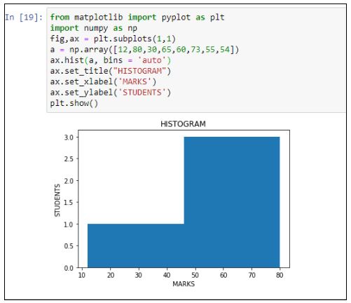
Let's watch a detailed explanation of what histograms are and how they differ from bar charts.

As you saw, the bins parameter is key. You can provide an integer for a set number of equal-width bins, or a list of numbers to define the precise edges of each bin.

Here's a code example using ax.hist():

# 1. Prepare data (e.g., from a normal distribution)
data = np.random.randn(1000)




# 2. Create Figure and Axes
fig, ax = plt.subplots()




# 3. Plot the histogram
# Bins are crucial for histograms. Here, we ask for 30 bins.
ax.hist(data, bins=30, edgecolor='black')




# 4. Customize
ax.set_title('Distribution of a Sample Dataset')
ax.set_xlabel('Value')
ax.set_ylabel('Frequency')




# 5. Show plot
plt.show()

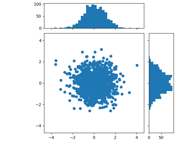
By combining these plot types, you can create rich dashboards. For instance, a scatter plot can show the relationship between two variables, while marginal histograms show their individual distributions.

5. Your Turn: Practice Exercise

Now it's time to apply what you've learned. We'll use the video game sales dataset from the previous lesson to create one of each plot type.

Task (15 minutes):

1. Run the initial code block to load the dataset and perform a simple aggregation, which we'll visualize.
2. Line Plot: The aggregated data sales_by_year contains the total global sales for each year. Create a line plot to visualize this trend over time.
3. Scatter Plot: Is there a relationship between how critics score a game (Critic_Score) and how users score it (User_Score)? Create a scatter plot to find out. Make sure to handle missing values by dropping them.
4. Histogram: What is the distribution of game release years? Create a histogram of the Year column. Choose an appropriate number of bins to see the distribution clearly.

# 1. Setup and Data Loading
import pandas as pd
import matplotlib.pyplot as plt




# Load the dataset
url = 'https://gist.githubusercontent.com/gwalker/8568092/raw/bb6ded017a3507973c1143c683fa6d4825595568/vgsales.csv'
df = pd.read_csv(url)




# Clean and aggregate data for the line plot
df_cleaned = df.dropna(subset=['Year'])
df_cleaned['Year'] = df_cleaned['Year'].astype(int)
sales_by_year = df_cleaned.groupby('Year')['Global_Sales'].sum()




# --- Your code goes below ---




# 2. Line Plot of Global Sales by Year





# 3. Scatter Plot of Critic Score vs. User Score





# 4. Histogram of Game Release Years

# 1. Setup and Data Loading
import pandas as pd
import matplotlib.pyplot as plt
import numpy as np # Often needed for data manipulation




# Load the dataset
url = 'https://gist.githubusercontent.com/gwalker/8568092/raw/bb6ded017a3507973c1143c683fa6d4825595568/vgsales.csv'
df = pd.read_csv(url)




# Clean and aggregate data for the line plot
df_cleaned = df.dropna(subset=['Year'])
df_cleaned['Year'] = df_cleaned['Year'].astype(int)
sales_by_year = df_cleaned.groupby('Year')['Global_Sales'].sum()





# 2. Line Plot of Global Sales by Year
fig, ax = plt.subplots(figsize=(10, 5)) # Use a wider figure for time series
ax.plot(sales_by_year.index, sales_by_year.values)
ax.set_title('Total Global Video Game Sales by Year')
ax.set_xlabel('Year')
ax.set_ylabel('Total Sales (in millions)')
ax.grid(True)
plt.show()





# 3. Scatter Plot of Critic Score vs. User Score
# Clean data for this specific plot
score_df = df[['Critic_Score', 'User_Score']].dropna()



# 'User_Score' is an object type, need to convert to numeric, coercing errors
score_df['User_Score'] = pd.to_numeric(score_df['User_Score'], errors='coerce')
score_df = score_df.dropna()

fig, ax = plt.subplots()
ax.scatter(score_df['Critic_Score'], score_df['User_Score'], alpha=0.3)
ax.set_title('Critic Score vs. User Score')
ax.set_xlabel('Critic Score')
ax.set_ylabel('User Score')
plt.show()





# 4. Histogram of Game Release Years
# We can use the df_cleaned from before
fig, ax = plt.subplots()



# Let's create bins for every 2 years from 1980 to 2020
bins = np.arange(1980, 2021, 2)
ax.hist(df_cleaned['Year'], bins=bins, edgecolor='black')
ax.set_title('Distribution of Game Release Years')
ax.set_xlabel('Year')
ax.set_ylabel('Number of Games Released')
plt.show()

Conclusion

Congratulations on completing this lesson and the "Data Handling and Visualization" module! You are now equipped with the fundamental skills to take a dataset, clean it, aggregate it, and visualize the results.

Key Takeaways:

• Line Plots (ax.plot): Best for showing trends over a continuous sequence, like time.
• Scatter Plots (ax.scatter): Best for visualizing the relationship and correlation between two numerical variables.
• Histograms (ax.hist): Best for understanding the frequency distribution of a single numerical variable.
• Anatomy of a Plot: The Figure is the canvas, and the Axes is where you draw. Using the object-oriented style (fig, ax = plt.subplots()) gives you explicit control and leads to more readable code.

Preview of the Next Module:
So far, you have built a strong foundation in Python programming, from variables and loops to sophisticated data manipulation with pandas and visualization with Matplotlib. You have the practical tools to work with data.

To build truly intelligent systems—the core of your "Tony Stark" ambition—you also need to understand the principles of logical reasoning that form the bedrock of all computation, algorithms, and AI. In our next module, "Logic and Computational Thinking," we will pivot from writing code to exploring the formal rules of thought. We'll start with the most basic building blocks of logic: propositions and truth tables. This will give you the formal framework to reason about systems with the precision required for advanced AI.