Data Manipulation with pandas

1. What is a Pandas DataFrame?

Before we start loading data, it's crucial to understand what a DataFrame is and why it's so fundamental to data science in Python. While a NumPy array is a powerful tool for homogenous numerical data, a DataFrame is designed for heterogeneous, tabular data.

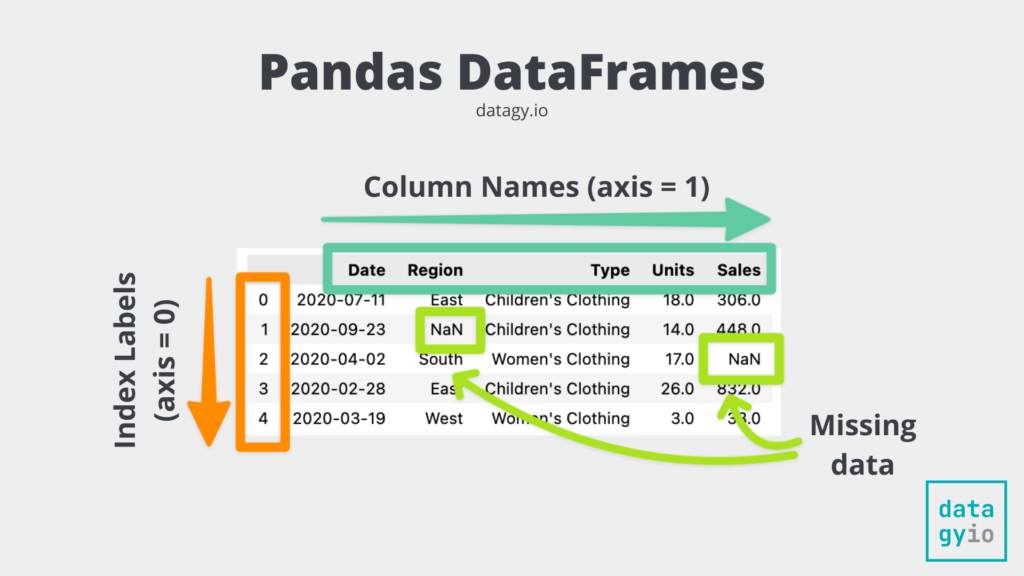
To build on your preference for a theory-first approach, let's read a short article that defines a DataFrame and explains its advantages.

In short, a DataFrame improves upon a NumPy array by providing:

• Labeled axes: You can refer to columns by name (e.g., 'age', 'price') and rows by a meaningful index, instead of just numbers.
• Heterogeneous data: Each column can have its own data type (e.g., numbers in one column, text in another), just like a spreadsheet.
• Rich functionality: It comes with a vast library of built-in functions for cleaning, transforming, aggregating, and visualizing data.

2. Loading Data into a DataFrame

While you can create a DataFrame from scratch (e.g., from Python dictionaries), the most common starting point is loading data from an external file. The most prevalent file format for tabular data is the CSV (Comma-Separated Values) file.

Pandas makes this incredibly simple with the pd.read_csv() function. You just need to provide the path to the file.

The following video demonstrates how to load data from various file types and discusses some of the practical considerations.

Here is an example of the code you just saw. To use it, you must first import the pandas library, conventionally aliased as pd.

import pandas as pd




# Load data from a local CSV file
df = pd.read_csv('path/to/your/file.csv')




# Or, load data directly from a URL
url = 'https://raw.githubusercontent.com/fivethirtyeight/data/master/college-majors/majors-list.csv'
df_majors = pd.read_csv(url)

3. Inspecting a DataFrame

Once you've loaded your data, the first step is always to inspect it to understand its structure, content, and quality. This initial exploration helps you check for issues like missing data, incorrect data types, or unexpected values.

Pandas provides several essential methods for a quick overview:

• .head(n): Shows the first n rows (default is 5).
• .tail(n): Shows the last n rows (default is 5).
• .info(): Provides a concise summary, including the number of entries, the data type of each column, and the number of non-null values. This is extremely useful for spotting missing data.
• .describe(): Generates descriptive statistics for numerical columns (count, mean, standard deviation, min, max, etc.).
• .shape: Returns a tuple representing the dimensions of the DataFrame (rows, columns).
• .columns: Displays the column labels.

Let's watch a short clip that demonstrates these fundamental inspection tools.

4. Selecting Data

After inspecting the data, you'll need to select specific parts of it for analysis. Pandas offers a powerful and flexible set of tools for this, which can be broadly categorized into three types of selection.

a) Selecting Columns

You can select a single column using bracket notation, which returns a pandas Series (a 1D labeled array). To select multiple columns, you pass a list of column names inside the brackets, which returns a new DataFrame.

# Select a single column (returns a Series)
major_category_series = df_majors['Major_category']




# Select multiple columns (returns a DataFrame)
# Note the double brackets!
subset_df = df_majors[['Major', 'Major_category']]

b) Selecting Rows with .loc and .iloc

This is one of the most powerful and often confusing aspects of pandas for newcomers. It's vital to understand the difference:

• .loc is for label-based selection. It uses the index labels to select rows.
• .iloc is for integer position-based selection. It uses the integer position of rows (starting from 0), just like slicing a Python list.

c) Selecting Data with Conditions (Boolean Indexing)

This is the most common way to filter data. You create a boolean condition (e.g., df['age'] > 30) and use it to select only the rows where the condition is True.

# Find all majors in the 'Engineering' category
engineering_majors = df_majors[df_majors['Major_category'] == 'Engineering']




# You can combine conditions using & (and) and | (or).
# Note: Each condition must be wrapped in parentheses.
stem_and_high_paying = df_majors[(df_majors['Major_category'] == 'Engineering') | (df_majors['Major_category'] == 'Physical Sciences')]

The following video covers both .loc/.iloc and conditional filtering in detail.

Your Turn: Practice Exercise

Let's put this all together. You'll use a dataset of video game sales.

Task (5-10 minutes):

1. Run the code below to load a dataset of video game sales into a DataFrame named df_vgsales.
2. Inspect the DataFrame:
   • Display the first 7 rows.
   • Get a summary of the data types and non-null values for each column.
3. Select data:
   • Create a new DataFrame called nintendo_games that contains only the games published by 'Nintendo'.
   • From the original df_vgsales, select the row at position 100 using .iloc.
   • The index of this DataFrame is just the default integer index. Select the row with the label 100 using .loc. What do you notice?
   • Create a new DataFrame called popular_wii_games that contains games for the 'Wii' platform with more than 5 million sales in North America (NA_Sales).

# 1. Load the dataset
import pandas as pd
url = 'https://gist.githubusercontent.com/gwalker/8568092/raw/bb6ded017a3507973c1143c683fa6d4825595568/vgsales.csv'
df_vgsales = pd.read_csv(url)

import pandas as pd




# 1. Load the dataset
url = 'https://gist.githubusercontent.com/gwalker/8568092/raw/bb6ded017a3507973c1143c683fa6d4825595568/vgsales.csv'
df_vgsales = pd.read_csv(url)




# 2. Inspect the DataFrame
print("--- First 7 rows ---")
print(df_vgsales.head(7))

print("\n--- DataFrame Info ---")
df_vgsales.info()




# 3. Select data
# Create a new DataFrame with only Nintendo games
nintendo_games = df_vgsales[df_vgsales['Publisher'] == 'Nintendo']
print("\n--- Nintendo Games (first 5) ---")
print(nintendo_games.head())




# Select the row at position 100
row_at_position_100 = df_vgsales.iloc[100]
print("\n--- Row at position 100 (.iloc[100]) ---")
print(row_at_position_100)




# Select the row with label 100
row_with_label_100 = df_vgsales.loc[100]
print("\n--- Row with label 100 (.loc[100]) ---")
print(row_with_label_100)



# Notice: In this specific case, since the DataFrame has a default integer index
# starting from 0, .iloc[100] and .loc[100] select the exact same row.
# This is not always the case if the index is non-numeric or has been changed.




# Create a DataFrame of popular Wii games
popular_wii_games = df_vgsales[(df_vgsales['Platform'] == 'Wii') & (df_vgsales['NA_Sales'] > 5)]
print("\n--- Popular Wii Games in North America ---")
print(popular_wii_games)

Conclusion

Fantastic work! You have just taken a major step in your journey. You've moved from the world of pure numerical arrays into the structured, labeled world of DataFrames, which is how most real-world data analysis begins.

Key Takeaways:

• A DataFrame is a 2D, labeled, and heterogeneous data structure, making it ideal for tabular data.
• You can easily load data from files like CSVs using pd.read_csv().
• Inspecting data with .head(), .info(), and .describe() is the critical first step to understanding your dataset.
• You can select data by:
  • Columns: using df['column_name'].
  • Rows by label: using .loc[].
  • Rows by position: using .iloc[].
  • Conditions: using boolean indexing like df[df['column'] > value].

Preview of the Next Lesson:
In our next lesson, we will step back slightly to look at a core Python feature that is extremely useful when working with pandas: list comprehensions. You'll learn how to "Write list comprehensions to create and transform lists concisely." This powerful technique allows you to create and modify lists in a single, readable line of code. It's a fundamental tool for preparing data before it enters a DataFrame or for creating new columns based on complex logic—a key skill for writing the clean, efficient code expected of a top-tier developer.