Eigenvalues and Eigenvectors: A Geometric Perspective

1. The Core Geometric Idea: Invariant Directions

A linear transformation can be thought of as a process that moves and reshapes vector space. It might stretch, shrink, shear, or rotate vectors. In this storm of movement, eigenvectors are the calm at the center.

An eigenvector of a transformation is a non-zero vector whose direction is unchanged by the transformation. It might get longer, shorter, or even flip to point in the opposite direction, but it remains on the same line through the origin (its "span"). This line is an invariant direction of the transformation.

The eigenvalue is the factor by which the eigenvector is stretched or shrunk.

• If $|\lambda |>1$, the eigenvector is stretched.
• If $|\lambda |<1$, the eigenvector is shrunk.
• If $\lambda <0$, the eigenvector is flipped and points in the opposite direction.
• If $\lambda =1$, the eigenvector is left unchanged.

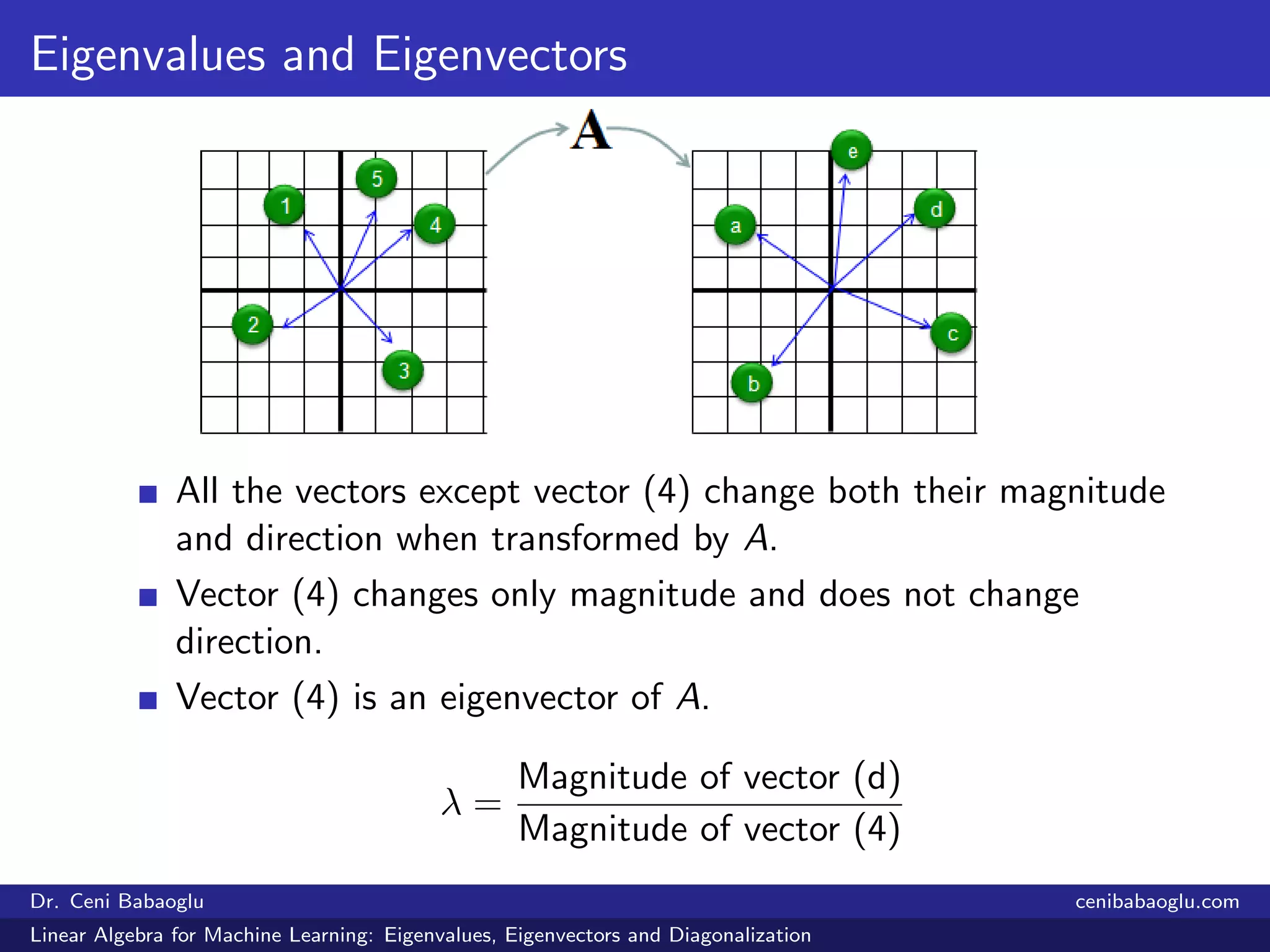
To get a feel for this, the following interactive visualization is excellent.

2. Deepening the Intuition with 3Blue1Brown

Now that you have a hands-on feel for the concept, let's refine this understanding with some of the best visualizations in mathematics. We'll return to the 3Blue1Brown video from our last lesson, but this time, your focus should be entirely on the geometric narrative.

As the video shows, identifying the eigenvectors of a transformation helps reveal its fundamental properties, which might be hidden in the raw numbers of the matrix. Thinking about a 3D rotation in terms of its axis (an eigenvector) and an angle is far more intuitive than trying to interpret a 3x3 matrix.

3. A Gallery of Transformations

A robust mental model must account for variety. What do eigenvalues and eigenvectors look like for transformations that aren't simple stretches? Let's consider a few important cases. Your computational work from the last lesson will connect directly to the geometry here.

• Rotation (in 2D): A pure rotation, for example by 90 degrees, changes the direction of every non-zero vector. Geometrically, there are no invariant lines. Algebraically, as you saw before, the characteristic equation (e.g., ${\lambda }^2+1=0$) has no real solutions. The algebra confirms the geometry.

• Shear: A shear transformation slides layers of space past one another. In a standard horizontal shear, only vectors on the x-axis remain on their span (with an eigenvalue of 1). There are no other invariant directions. This corresponds to the algebraic result of finding only one eigenvalue and one line of eigenvectors.

• Scaling: A transformation that scales everything uniformly by a factor of, say, 2, is special. Every vector is an eigenvector because every vector stays on its span, stretched by a factor of 2. In this case, there is only one eigenvalue ($\lambda =2$), but the entire plane is the eigenspace.

The following video segment and text will solidify your understanding of these cases.

For a quick review of these specific cases, the text version is also very helpful.

4. The Eigenbasis: A Natural Coordinate System

We now arrive at the most powerful concept in this lesson. What if a transformation has enough eigenvectors, pointing in different directions, that we can use them to define our entire coordinate system?

This set of eigenvector basis vectors is called an eigenbasis.

When you describe a transformation from the perspective of its eigenbasis, it becomes incredibly simple. All the complex shearing and rotating disappears. The transformation is revealed to be nothing more than simple scaling along each of the new basis axes. The matrix for the transformation becomes a diagonal matrix, with the eigenvalues as its diagonal entries.

This is a profound idea: by changing our coordinate system to one that is "natural" to the transformation, we can understand its action in the simplest way possible. This is a recurring theme in physics and engineering—and especially in machine learning, where changing basis (e.g., using PCA) is a fundamental tool for simplifying complex data.

Conclusion

In this lesson, we moved beyond calculation to build a strong geometric intuition for eigenvalues and eigenvectors. You have seen that they represent the deep structure of a linear transformation—its intrinsic "axes" of action.

Key Takeaways:

• Eigenvectors point in the directions that a transformation does not alter, representing the invariant lines or eigenspaces.
• Eigenvalues are the scaling factors along these invariant directions, telling you if vectors are stretched, shrunk, or flipped.
• The geometric properties of a transformation (like rotation, shear, or scaling) are directly reflected in its set of eigenvalues and eigenvectors.
• An eigenbasis is a special coordinate system composed of eigenvectors. In this basis, the transformation's matrix becomes diagonal, simplifying its structure and making computations like matrix exponentiation trivial.

Preview of the Next Lesson:
We have now established a solid theoretical and geometric foundation for some key concepts in linear algebra. In the next lesson, we will pivot to practical application. You will learn to implement matrix operations and solve linear systems using NumPy, a fundamental Python library for numerical computing. This will be your first step in translating abstract mathematical concepts into concrete code, a skill essential for building AI systems.