Random Samples and Summary Statistics in Python

1. Generating Random Data: The Foundation of Simulation

In statistics and machine learning, we often need to generate random data. This can be for simulating experiments (like we did conceptually in the last lesson), initializing the weights of a neural network, or creating test data to validate our algorithms. The NumPy library is the standard for this in Python.

Historically, you might see code using functions like np.random.randint(). However, the modern and recommended best practice is to first create a random number generator object and then call methods on it. This offers better performance and statistical properties.

Let's watch a video that demonstrates this modern approach.

As the video explained, the process is straightforward:

1. Import NumPy: import numpy as np
2. Create a Generator: rng = np.random.default_rng(seed=42)
   • The seed is an arbitrary number. Using the same seed ensures you get the exact same sequence of "random" numbers every time you run the code. This is essential for debugging and creating reproducible scientific results.
3. Generate Numbers: Use methods on the rng object.

Here's a quick code summary:

import numpy as np




# Create a random number generator with a seed for reproducibility
rng = np.random.default_rng(seed=42)




# Generate 5 random integers between 1 and 10 (exclusive of 11)
random_integers = rng.integers(low=1, high=11, size=5)
print(f"Random integers: {random_integers}")




# Generate an array of 4 random floats between 0 and 1
random_floats = rng.random(size=4)
print(f"Random floats (uniform distribution): {random_floats}")

Sampling from Specific Distributions

While generating random integers and uniform floats is useful, we often need to simulate data that follows a specific statistical distribution. Given our previous lessons, the most important one is the normal distribution.

The generator object has a normal() method for this purpose.

• rng.normal(loc, scale, size)
  • loc: The mean ($\mu$) of the distribution.
  • scale: The standard deviation ($\sigma$) of the distribution.
  • size: The number of samples to generate.

Let's generate data that looks like it came from a population with a mean of 100 and a standard deviation of 15 (like IQ scores).

# Generate 1000 samples from a normal distribution with mean=100 and std=15
iq_scores = rng.normal(loc=100, scale=15, size=1000)




# We can see the first 5 generated scores
print(f"First 5 simulated IQ scores: {iq_scores[:5]}")

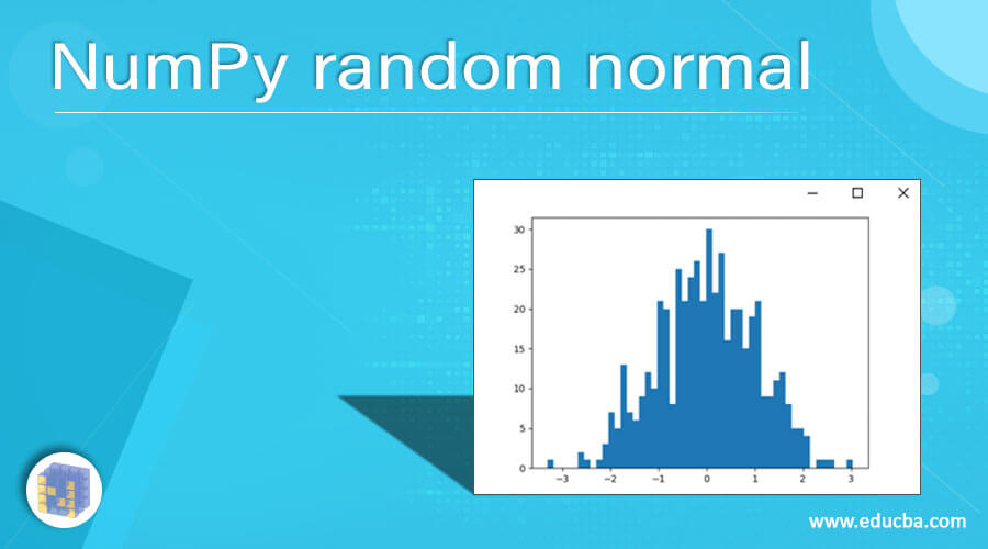
When you generate many samples from a normal distribution, their histogram will resemble the classic bell curve.

2. Computing Summary Statistics

Now that we have a sample, what can we do with it? The first step in any data analysis is to compute summary statistics (or descriptive statistics). These are single numbers that summarize the key characteristics of the dataset, such as its central tendency and spread.

The NumPy Approach

NumPy provides fast and efficient functions for these calculations. Let's explore them.

Let's apply these functions to the iq_scores we generated earlier.

# Use the iq_scores array from the previous step
sample_mean = np.mean(iq_scores)
sample_std = np.std(iq_scores)
sample_min = np.min(iq_scores)
sample_max = np.max(iq_scores)

print(f"Sample Mean: {sample_mean:.2f}")
print(f"Sample Std Dev: {sample_std:.2f}")
print(f"Sample Min: {sample_min:.2f}")
print(f"Sample Max: {sample_max:.2f}")

You'll notice that the sample mean and standard deviation are very close, but not exactly equal, to the loc=100 and scale=15 we specified. This is a perfect demonstration of sampling variability, a concept we've discussed in previous lessons.

The Pandas Approach

While NumPy is excellent for raw numerical operations, the Pandas library (which you were introduced to in Module 2) is often more convenient for statistical analysis. It builds on NumPy and provides data structures with helpful labels and even more powerful summary methods.

The standout feature in Pandas is the .describe() method. It provides a full suite of summary statistics with a single command. Let's try it with our iq_scores. First, we'll put our NumPy array into a Pandas Series object.

import pandas as pd




# Create a Pandas Series from our NumPy array
iq_series = pd.Series(iq_scores)




# Get the full descriptive statistics summary
summary = iq_series.describe()

print(summary)

Running this code gives you the count, mean, standard deviation, min, max, and the quartiles (25%, 50%, 75%) all at once. This is an incredibly efficient way to get a first look at any dataset.

3. Application: A Mini-Simulation

Let's tie this all together by revisiting the scenario from our previous lesson on hypothesis testing.

Scenario Recap: A researcher claimed college students spend at least 15 hours per week on social media ($H_0:\mu \ge 15$). Our test sample of 100 students had a mean of 14.4 hours.

Let's use our new skills to simulate what happens if the true population mean really was, for example, 14.5 hours with a standard deviation of 3.25 hours. What would a random sample from this population look like?

Your Task:

1. Use np.random.default_rng() to create a generator.
2. Generate a simulated sample of 100 students from a normal distribution where the true mean (loc) is 14.5 and the true standard deviation (scale) is 3.25.
3. Calculate the mean of your generated sample.
4. Run your code a few times. Does the sample mean come out to be exactly 14.5 every time? Why or why not?

This exercise simulates the act of data collection and directly illustrates how a sample is a noisy but informative snapshot of a larger population. The slight variations you see in the sample mean upon each run are the essence of sampling error.

# Step 1: Create a generator
rng_sim = np.random.default_rng() # No seed, so it's different each time!




# Step 2: Generate a sample
true_mean = 14.5
true_std = 3.25
sample_size = 100
simulated_sample = rng_sim.normal(loc=true_mean, scale=true_std, size=sample_size)




# Step 3: Calculate the sample mean
simulated_mean = np.mean(simulated_sample)

print(f"The true population mean was {true_mean}.")
print(f"Our simulated sample of {sample_size} students has a mean of {simulated_mean:.2f}.")

Conclusion

In this lesson, you have mastered the practical Python skills that bring statistical theory to life. You now have the power to create data and analyze it, a fundamental loop in all of data science and AI.

Key Takeaways:

• You can generate random numbers in Python using np.random.default_rng(), which is the modern standard for creating high-quality random data.
• The seed parameter is vital for creating reproducible experiments and simulations.
• You can simulate data from various distributions, including uniform (rng.random) and normal (rng.normal), by specifying parameters like loc (mean) and scale (std dev).
• You can compute summary statistics efficiently using either NumPy functions (e.g., np.mean()) or the more comprehensive Pandas .describe() method.

Preview of the Next Lesson:
You have now completed the "Probability and Statistics for AI" module. You've built a solid foundation, from understanding probability and distributions to testing hypotheses and now, implementing these concepts in code. With these tools in hand, you are ready to tackle the main event. In our next lesson, we will begin the "Foundations of Machine Learning" module, where you will learn to define machine learning and distinguish it from traditional programming. It's time to start building intelligent systems.