Understanding Hashing and Collision Resolution

1. The Quest for Constant-Time Search

We've seen that searching in an unsorted array takes $O(N)$ time, while a sorted array allows for $O(\log N)$ binary search. Can we do even better? The driving motivation behind hashing is to achieve an average search time of $O(1)$.

The following video provides an excellent introduction to this idea. It starts by comparing hashing to linear and binary search and then introduces the core concept of mapping a key directly to an array index.

As the video explained, the core components of hashing are:

• Hash Table: An array that stores the data.
• Key: The data (or an identifier for the data) we want to store or retrieve.
• Hash Function: A function that takes a key and computes an index in the hash table. A simple example is h(key) = key % table_size.
• Collision: The scenario where two different keys map to the same index. Since collisions are practically unavoidable, handling them effectively is crucial.

2. What Makes a Good Hash Function?

A good hash function is the cornerstone of an efficient hash table. It should have two main properties:

1. Fast Computation: It must be quick to calculate. If the hash function itself is slow, it defeats the purpose of aiming for $O(1)$ operations. For strings, this is often $O(L)$ where $L$ is the length of the string.
2. Uniform Distribution: It should spread keys as evenly as possible across the available indices to minimize collisions.

Your experience with various programming languages and projects gives you a good footing to understand how different data types can be hashed.

In Java, the hashCode() method provides the integer hash code for an object. This hash code is then typically mapped to a valid index in the hash table array, often using a modulo operation or bitwise tricks. For your custom classes, it's essential to correctly override both hashCode() and equals() to ensure they work correctly in hash-based collections like HashMap and HashSet.

3. Collision Resolution Strategies

Since even the best hash functions can produce collisions, we need robust strategies to handle them. There are two main families of techniques.

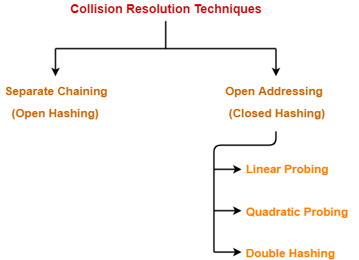
Let's explore each branch.

A) Separate Chaining (or Open Hashing)

This is the most straightforward and common strategy. The idea is to make each slot in the hash table a "bucket" that can hold multiple elements. This bucket is typically implemented as a linked list.

When a key is hashed to an index:

• Insertion: You add the new key-value pair to the linked list at that index. This is an $O(1)$ operation if you add to the head of the list.
• Search/Deletion: You traverse the linked list at that index to find the key. The time complexity depends on the length of the list.

The performance of this method depends on the load factor, $\lambda$, defined as:
$\lambda =\frac{n}{m}=\frac{\text{number of elements}}{\text{number of slots}}$

The average length of a chain is $\lambda$, so the average time for search and delete is $O(\lambda )$. If we keep the load factor low (e.g., by resizing the table when $\lambda$ gets too high), the performance remains effectively constant, $O(1)$.

A key optimization in modern Java (HashMap since version 8) is that if a linked list at a bucket grows too long (e.g., beyond 8 elements), it is converted into a self-balancing binary search tree. This improves the worst-case lookup time for that bucket from $O(n)$ to $O(\log n)$.

B) Open Addressing (or Closed Hashing)

In this strategy, all elements are stored directly within the hash table itself. If a collision occurs at index i, we "probe" or search for the next available slot according to a fixed sequence.

The three main probing methods are:

1. Linear Probing: If h(key) is occupied, try h(key) + 1, then h(key) + 2, and so on, wrapping around the table if necessary.

   • Formula: (h(key) + i) % m for i = 0, 1, 2, ...
   • Problem: This leads to primary clustering, where long runs of occupied slots build up, significantly degrading performance as searches have to traverse these clusters.

2. Quadratic Probing: To mitigate clustering, the probe sequence jumps quadratically. If h(key) is occupied, try h(key) + 1^2, then h(key) + 2^2, and so on.

   • Formula: (h(key) + i^2) % m for i = 0, 1, 2, ...
   • Problem: This avoids primary clustering but can suffer from secondary clustering, where keys that initially hash to the same location follow the exact same probe sequence.

3. Double Hashing: This method uses a second, independent hash function to determine the step size for the probe sequence, effectively eliminating both primary and secondary clustering.

   • Formula: (h1(key) + i * h2(key)) % m for i = 0, 1, 2, ...

The following video and article explain these techniques clearly.

4. Comparison: Chaining vs. Open Addressing

Knowing the trade-offs between these two strategies is a classic interview topic.

Here's a summary of the most important points:

• Space: Chaining uses extra space for pointers in the linked lists. Open addressing uses all space within the table itself.
• Cache Performance: Open addressing has better cache locality because all elements are in a contiguous array, which CPUs can cache effectively. Chaining can be slow as linked list nodes may be scattered in memory.
• Deletion: Deletion is simple in chaining (remove from list). In open addressing, it's complex; you can't just empty a slot, as it might break a probe chain for other elements. You must mark it with a special "deleted" value.
• Load Factor: Chaining works well even with $\lambda >1$. Open addressing requires $\lambda <1$ and its performance degrades sharply as $\lambda$ approaches 1.

In practice, Separate Chaining is used more often (it's the basis for Java's HashMap), largely due to its simpler implementation and more graceful performance degradation as the table fills up.

Conclusion

You've now covered the theoretical foundation of hashing. This is a critical first step, and these concepts are frequently tested in interviews.

Key Takeaways:

• Hashing aims to provide $O(1)$ average time for search, insertion, and deletion by mapping keys directly to array indices.
• A good hash function is fast and distributes keys uniformly to minimize collisions.
• Collisions are inevitable and are handled by two main strategies:
  • Separate Chaining: Each table slot is a bucket (like a linked list) for colliding keys. It's simple and handles high load factors well.
  • Open Addressing: Colliding keys are placed in other empty slots within the table using a probe sequence (linear, quadratic, or double hashing). It has better cache performance but is more complex to implement and sensitive to load factor.

Preview of the Next Lesson:
Theory is great, but your goal is to excel in practical coding interviews. In the next lesson, you will put this knowledge into practice by implementing a hash table from scratch using the Separate Chaining method in Java. This will solidify your understanding and prepare you for a common hands-on interview task.