3D Math for Physics Engines

Welcome back to our journey of building a physics engine from the ground up. In the last lesson, we established a crucial tool for visual feedback: a debug-drawing system. This system allows us to render simple geometry, giving us a window into the otherwise invisible workings of our engine. Now that we can see things, it's time to create the mathematical objects that our engine will see and manipulate: vectors and matrices.

This lesson is dedicated to implementing a core 3D math library. For a physics engine, this is the equivalent of forging the fundamental tools and materials—everything from position and velocity to orientation and force will be represented and transformed using the components we build today. Given your familiarity with linear algebra, we will focus on the practical C++ implementation details and design choices that lead to a robust, efficient, and clear math library tailored for physics simulation. We will build our own vec3, vec4, and mat4 types and equip them with the essential operations that will power every subsystem of our engine.

Designing a Vector Math Library

Before we start writing code, it's worth considering the design of a good math library. It needs to be performant, flexible, and intuitive to use. A fantastic blog post by Nathan Reed, "On Vector Math Libraries," outlines several best practices that we can adopt.

On Vector Math Libraries – Nathan Reed's coding blog

This article discusses high-level design principles for vector and matrix libraries in C++. It provides the "why" behind many of the implementation choices we'll make.

Please read the introduction and the following key sections: Parameterize By Dimension: This section makes the case for generic, templated implementations and introduces a very useful union technique to provide named components (like .x, .y) for our vectors. We will use this technique directly. Operations: Focus on the philosophy presented here regarding operator overloading (using them for component-wise operations) and the preference for free functions like dot(a, b) over member functions like a.dot(b).

The key takeaways from this reading are that we should strive for a clean, consistent API. While we will implement concrete vec3 and mat4 types using float for our 3D engine, the principles of using unions for aliasing and a clear functional style for operations are directly applicable.

Implementing Vector Types

With these design principles in mind, let's get to the implementation. We'll start with the most fundamental object in 3D physics: the vector. A video from Travis Vroman's "Kohi Game Engine" series provides an excellent, practical walkthrough of creating these types in C. We'll adapt this C-style implementation to fit our C++ context.

Kohi #022: Build System Update and Math Library Part 1 (Vulkan Game Engine Series)

This video provides a step-by-step guide to implementing vector types, demonstrating the union trick and covering the core data structures we need.

First, watch the segment on 2D vectors from this point. Pay close attention to how a union is used to allow a vector's components to be accessed as x/y, r/g, u/v, or as an array elements[0]/elements[1]. Next, watch the explanation of 3D vectors from here. This extends the vec2 concept to the vec3 we will use most frequently. Finally, review the section on 4D vectors from here. The video explains the crucial role of the fourth component, w, in distinguishing between a point in space (w=1) and a direction vector (w=0). This distinction is fundamental for applying transformations correctly.

The `vec3` Type

Let's start by defining our vec3 structure based on these ideas. It will represent positions, velocities, accelerations, forces, and more.

struct vec3 {
    union {
        struct {
            float x, y, z;
        };
        struct {
            float r, g, b;
        };
        float elements[3];
    };
};

Now, let's implement the essential operations for vec3. These should be implemented as free functions. The video provides a clear guide for the implementation of all these functions.

Kohi #022: Build System Update and Math Library Part 1 (Vulkan Game Engine Series)

This part of the video details the implementation of all the essential vec3 functions.

Watch from this section which covers the implementation for vec3 functions. You should implement the following, referring to the video for the exact logic: Creation: vec3_zero(), vec3_one(), and specific directional vectors like vec3_up() and vec3_forward(). Arithmetic: vec3_add(), vec3_sub(), vec3_mul() (component-wise), vec3_div(), and a version that multiplies by a scalar. Length: vec3_length_squared() and vec3_length(). It's vital to have the squared version for performance, as it avoids a costly square root operation and is sufficient for many comparisons. Normalization: vec3_normalize(). This produces a unit vector, which is essential for representing directions. Dot Product: vec3_dot(). This operation is critical for calculating projections and determining the angle between two vectors. For instance, it's used to determine how much of a velocity vector is aligned with a contact normal. Cross Product: vec3_cross(). The cross product of two vectors produces a third vector that is orthogonal to both. In physics, this is the fundamental operation for calculating torque: \vec{\tau} = \vec{r} \times \vec{F}, where \vec{r} is the vector from the center of mass to the point of force application.

Implementing Matrix Types

Vectors represent quantities in space, but matrices are what allow us to manipulate and transform them. For our 3D engine, the 4x4 matrix, or mat4, is the workhorse. It can encode an object's complete orientation and position (its "transform") and is used to move vectors and points between different coordinate systems, like from an object's local "body space" to the shared "world space".

The classic text "An Introduction to Physically-Based Modeling" by Baraff and Witkin demonstrates exactly why we need these matrix operations.

[PDF] An Introduction to Physically Based Modeling: Rigid Body ...

This document provides the theoretical underpinnings for rigid body physics and shows where matrix and vector math are applied.

Skim the sections from Position and Orientation up to The Inertia Tensor. Don't worry about memorizing the physics derivations. Instead, focus on identifying the matrix and vector operations used. You will see: Matrix-vector multiplication to transform points: p(t) = R(t)p0 + x(t). The * operator, a matrix form of the cross product: a x b = a*b. Matrix-matrix multiplication: ˙R(t) = ω(t)*R(t). Matrix transpose in the inertia tensor update: I(t) = R(t)IbodyR(t)T.

This reading confirms the necessity of implementing a robust mat4 type. Let's return to Travis Vroman's video series for the practical implementation.

Kohi #023: Math Library Part 2: Matrices and Quaternions (Vulkan Game Engine Series)

This follow-up video covers the implementation of the mat4 type and its core operations.

Watch the introduction from the beginning to understand the structure of a 4x4 matrix. Implement the mat4 identity function, as shown from this segment. The identity matrix is the starting point for all other transformations. The most important matrix operation is multiplication. Watch from here to implement it. This is how we will combine scale, rotation, and translation into a single transform matrix. You will also need functions to create specific transformation matrices. Implement mat4_translation (from here) and mat4_scale (from here). Finally, implement mat4_transpose (from this part) and mat4_inverse (from this part). As we saw in the Baraff paper, transpose is needed for updating the inertia tensor, and inverse is needed for converting angular momentum to angular velocity.

Matrix-Vector Multiplication

The videos focus on matrix-matrix multiplication. You must also implement a function to multiply a mat4 by a vec4. This is how we actually apply a transformation to a point or vector.

The rule for multiplying a matrix M by a column vector v to get a new vector v' is:
v'_i = M_i0*v_0 + M_i1*v_1 + M_i2*v_2 + M_i3*v_3 for each row i of the matrix.

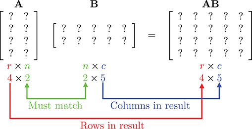
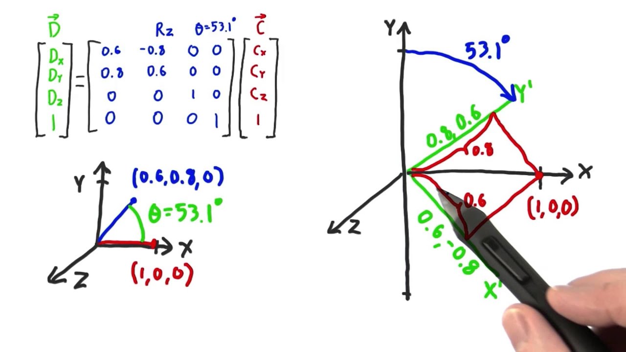
This diagram shows the dimensional rule for matrix-matrix multiplication. A similar rule applies to matrix-vector multiplication, where a 4x4 matrix multiplied by a 4x1 vector results in a 4x1 vector.

Your mat4_mul_vec4 function will take a matrix and a vec4 and return the transformed vec4. Remember the distinction between points and vectors: a point (x, y, z, 1) will be translated by the matrix, whereas a direction vector (x, y, z, 0) will not. Your matrix multiplication implementation will handle this correctly automatically.

A visual example of a 4x4 rotation matrix being applied to a vector `C` to produce a new, rotated vector `D`. This is the core operation for changing an object's orientation.

Putting It All Together

You now have the data structures and functions for a basic but powerful math library. I encourage you to use the debug-drawing system from our previous lesson to visualize your work.

Create a vec3 representing a position and another representing a velocity. Use DrawLine to draw the velocity vector originating from the position.
Create a mat4 translation matrix and use it to define a transform. Use your DrawTransform function to visualize the coordinate system at that new position.
Combine a rotation (you can manually create a simple one for now) and a translation matrix through multiplication, and visualize the resulting transform.

This practice will build confidence in your library and give you immediate visual feedback that your math is working correctly.

Conclusion

In this lesson, we have constructed the mathematical bedrock of our physics engine. We designed and implemented vec3, vec4, and mat4 types, along with the essential operations needed to manipulate them.

Key Takeaways:

A well-designed math library uses C++ features like unions to create flexible and readable code.
Vectors (vec3) are used to represent physical quantities like position, velocity, and force.
Matrices (mat4) are used to represent transformations (rotation, translation, scale) and to convert points and vectors between different coordinate systems.
Core vector operations include arithmetic, length, normalization, and the dot and cross products, each with a specific physical application.
Core matrix operations include multiplication (for combining transforms), inverse (for undoing transforms), and transpose.
The w component of a vec4 is a powerful tool for distinguishing between points (w=1) and direction vectors (w=0) in affine transformations.

We now have the tools to represent an object's state. In the next lesson, we will focus specifically on orientation. We'll explore different ways to represent 3D rotations—axis-angle, rotation matrices, and quaternions—and implement the functions to convert between them, solidifying the foundation for simulating rotating rigid bodies.

Recommended resources