Inspecting DataFrame Properties and Selecting Data

1. First Look: Inspecting Your DataFrame

Before you start any serious analysis, you need to get a feel for your dataset. What does it look like? How big is it? What kind of data does it contain? Pandas provides a suite of simple but powerful attributes and methods for this initial inspection.

The video below gives a great tour of these essential tools.

Let's recap the most important methods you just saw:

• .head(n) and .tail(n): Show the first or last n rows (default is 5). This is the quickest way to see a sample of your data and its structure.
• .shape: An attribute (not a method, so no parentheses) that returns a tuple representing the dimensionality of the DataFrame: (number_of_rows, number_of_columns).
• .info(): Provides a concise summary. It's especially useful for checking the data type (Dtype) of each column and finding columns with missing values (by comparing the Non-Null Count to the total number of entries).
• .describe(): Generates descriptive statistics for the numerical columns, such as count, mean, standard deviation, min, max, and percentiles. This is a great way to get a quick sense of the distribution and scale of your numerical data.

The official Pandas guide, "10 minutes to pandas," also provides a good summary of these functions.

2. Selecting Data: loc, iloc, and []

Once you have a high-level overview, you'll need to select specific subsets of your data. This is where Pandas' indexing capabilities shine. However, the different options can be confusing for beginners. We'll focus on a clear, consistent approach.

The three primary ways to select data are:

1. [] (Bracket notation): Good for quick column selection.
2. .loc: For label-based selection.
3. .iloc: For integer position-based selection.

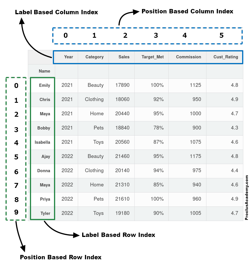
This image clearly illustrates the difference between label-based and position-based indexing, which is the core concept separating .loc and .iloc.

For a robust and readable approach, it's best to follow this simple rule:

Use .loc for labels and .iloc for positions. Always be explicit about selecting both rows and columns.

The following video provides an excellent, minimalist guide that champions this exact philosophy.

Now, let's break down each method with examples. We'll use the DataCamp article "Iloc vs Loc in Pandas" as our guide. It provides clear explanations and examples for both methods.

A. Selecting Columns with []

The simplest way to select one or more columns is with bracket notation.

• To select a single column, pass the column name as a string. The result is a Pandas Series.

  # Assume 'df' is a DataFrame with student data
  major_series = df['Major'] 
  

• To select multiple columns, pass a list of column names. The result is a new DataFrame.

  student_info_df = df[['Student', 'Grade']]
  

While you can use [] to slice rows (e.g., df[0:3]), this can be ambiguous. For clarity, it's better to use .loc or .iloc for any row selection.

B. Label-Based Selection with .loc

Use .loc when you want to select data using the index labels and column names. The syntax is df.loc[row_labels, column_labels].

• Select a single row: df.loc['row_label']
• Select multiple rows: df.loc[['row_label_1', 'row_label_2']]
• Select a slice of rows: df.loc['start_label':'end_label'] (Note: both endpoints are included).
• Select a single value: df.loc['row_label', 'column_label']
• Select rows and columns simultaneously: df.loc['start_label':'end_label', ['col1', 'col2']]

Boolean Indexing (a very powerful feature of .loc):
One of the most common uses of .loc is to select rows based on a condition. You can pass a boolean Series (a list of True/False values) as the row selector.

# Select all students who are CS majors
cs_majors_df = df.loc[df['Major'] == 'CS']

# Select all students with a grade above 90
high_achievers_df = df.loc[df['Grade'] > 90]

# Combine conditions (use & for AND, | for OR)
# Note the parentheses around each condition are required!
cs_high_achievers = df.loc[(df['Major'] == 'CS') & (df['Grade'] > 90)]

C. Position-Based Selection with .iloc

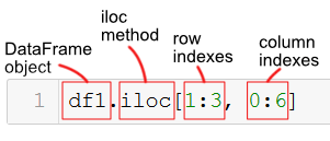
Use .iloc when you want to select data using integer positions (starting from 0). The syntax is df.iloc[row_positions, column_positions].

• Select a single row: df.iloc[0] (the first row)
• Select multiple rows: df.iloc[[0, 2, 5]]
• Select a slice of rows: df.iloc[0:3] (selects rows at position 0, 1, and 2. The endpoint is excluded, just like in standard Python slicing).
• Select a single value: df.iloc[0, 1] (value at the first row, second column)
• Select rows and columns simultaneously: df.iloc[0:3, [0, 2]] (first three rows, first and third columns)

         Major  Grade  Credits
Student                        
Alice       CS     85       90
Bob       Math     92      105
Charlie     CS     78       80
David  Physics     95      110

import pandas as pd

data = {'Major': ['CS', 'Math', 'CS', 'Physics'],
        'Grade': [85, 92, 78, 95],
        'Credits': [90, 105, 80, 110]}
index = ['Alice', 'Bob', 'Charlie', 'David']
df = pd.DataFrame(data, index=index)
df.index.name = 'Student'

# 1. Select the Grade for 'Bob' using .loc
bob_grade = df.loc['Bob', 'Grade']
print(f"Bob's grade: {bob_grade}\n")

# 2. Select the rows for 'Alice' and 'David' using .loc
alice_david_rows = df.loc[['Alice', 'David']]
print("Rows for Alice and David:\n", alice_david_rows, "\n")

# 3. Select the first two rows of the DataFrame using .iloc
first_two_rows = df.iloc[0:2] # or df.iloc[[0, 1]]
print("First two rows:\n", first_two_rows, "\n")

# 4. Select all students with more than 100 credits
high_credits = df.loc[df['Credits'] > 100]
print("Students with over 100 credits:\n", high_credits)

Conclusion

In this lesson, we covered the essential first steps of working with a new dataset in Pandas. You are now equipped to both inspect a DataFrame to understand its characteristics and to precisely select the data you need for your analysis.

Key Takeaways:

• Inspection is key: Always start by using .head(), .info(), and .describe() to get a quick understanding of your data's structure, types, and statistical properties.
• Choose the right tool for selection:
  • Use simple bracket notation df['column'] for quick, single-column selection.
  • Use .loc for label-based selection (names of rows/columns). It's great for slicing and powerful for conditional (boolean) filtering.
  • Use .iloc for integer-position-based selection (0-indexed). It behaves like standard Python list slicing.
• Be explicit: Using .loc and .iloc with both row and column selectors (df.loc[rows, cols]) leads to clearer and more predictable code.

Preview of the Next Lesson:
We've created DataFrames in memory and learned how to inspect and select from them. In the real world, data almost always comes from external files. In the next lesson, we will focus on the most common I/O (Input/Output) operations: loading data into DataFrames from files like CSV, Excel, and JSON, and exporting your processed DataFrames back to these formats.