Matrix Operations: Multiplication and Transposition

1. Matrix Multiplication: The Engine of Machine Learning

Matrix multiplication is more than just a computational procedure; it's the mathematical operation that underpins how information is transformed in most machine learning models. Unlike element-wise operations, it combines information from rows and columns in a very specific way.

The Fundamental Rule of Matrix Multiplication

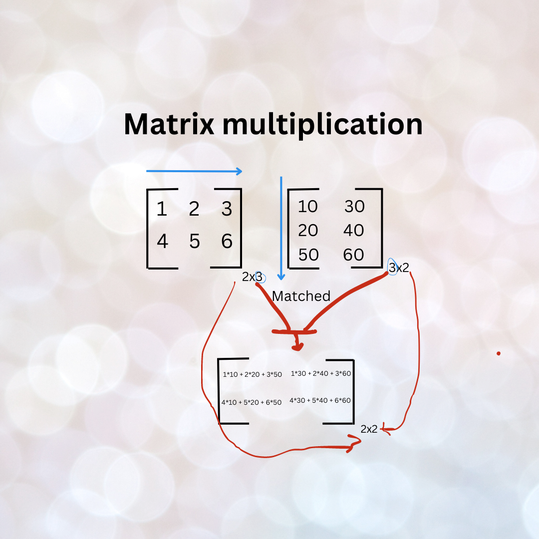
The first thing to learn about matrix multiplication is the rule for when it's possible. To multiply two matrices, the number of columns in the first matrix must equal the number of rows in the second matrix.

If you have a matrix $A$ with dimensions $(m\times n)$ and a matrix $B$ with dimensions $(n\times p)$, you can multiply them to get a new matrix $C$ with dimensions $(m\times p)$.

Each element in the resulting matrix $C$ is calculated by taking the dot product of a row from matrix $A$ and a column from matrix $B$.

A Step-by-Step Walkthrough

To see this process in action, let's watch a video that calculates a matrix-vector product (a special case of matrix multiplication) and then a full matrix-matrix product by hand.

Matrix Multiplication in NumPy

As you might expect, you don't need to implement this by hand in Python. NumPy provides a dedicated operator, @ (the "at" symbol), for matrix multiplication. This is the modern, recommended way to perform this operation. An older method, np.dot(), also works and you will see it in many codebases.

Let's use the examples from the video to perform the calculation in NumPy.

import numpy as np

# Matrix-vector multiplication example from the video
A_mv = np.array([[3, 4], 
                 [5, 6], 
                 [7, 8]])

B_mv = np.array([[1], 
                 [2]]) # Shape (2, 1) to be a column vector

# In the video, B was a 1D array. NumPy is flexible, but being explicit with shapes is good practice.
# B_mv_1d = np.array([1, 2])
# print(A_mv @ B_mv_1d) # This also works

C_mv = A_mv @ B_mv
print("Matrix-Vector Multiplication Result:")
print(C_mv)
print("-" * 20)

# Matrix-matrix multiplication example
A_mm = np.array([[3, 4], 
                 [5, 6], 
                 [7, 8]])

B_mm = np.array([[1, 9], 
                 [2, 0]])

C_mm = A_mm @ B_mm
print("Matrix-Matrix Multiplication Result:")
print(C_mm)

2. The Deeper Meaning: Multiplication as Transformation

So, what does matrix multiplication mean? From a geometric perspective, it represents applying one linear transformation after another. This is called the composition of transformations.

For example, you could have one matrix that represents a rotation and another that represents a shear. Multiplying them together creates a single new matrix that represents the combined effect of rotating and then shearing.

This is a profound insight that simplifies many complex ideas in linear algebra. Let's see it explained visually.

3. Properties of Matrix Multiplication

Understanding the properties of matrix multiplication is essential for correctly manipulating equations in machine learning.

• Not Commutative: This is perhaps the most important property. In general, $AB\ne BA$. The order matters! Thinking geometrically, rotating then shearing is not the same as shearing then rotating.
• Associative: The grouping of multiplication doesn't matter. $(AB)C=A(BC)$. Geometrically, this means applying transformation C, then B, then A is the same regardless of how you group the operations.
• Distributive: It distributes over addition. $A(B+C)=AB+AC$.
• Multiplicative Identity: There is an identity matrix $I$, which is a square matrix with 1s on the main diagonal and 0s elsewhere. For any matrix $A$, $AI=A$ and $IA=A$. It's the matrix equivalent of the number 1.

The text below summarizes these properties clearly.

4. Matrix Transposition

The transpose is a much simpler operation that rearranges a matrix's elements.

Definition and Calculation

The transpose of a matrix is obtained by swapping its rows and columns. The first row becomes the first column, the second row becomes the second column, and so on. The transpose of matrix $A$ is denoted as $A^T$.

If $A$ is an $(m\times n)$ matrix, then $A^T$ will be an $(n\times m)$ matrix.

Example:

In NumPy, you can get the transpose of an array using the .T attribute.

A = np.array([[1, 2, 3],
              [4, 5, 6]])

A_transpose = A.T

print("Original Matrix A (2x3):")
print(A)
print("\nTransposed Matrix A.T (3x2):")
print(A_transpose)

To learn more about the properties and some nuances of transposition, please review the following resource.

Key Properties of the Transpose

As detailed in the article, the transpose has several important properties. The most critical one for machine learning is the transpose of a product:

$(AB{)}^T=B^T{A}^T$

Notice that the order of the matrices is reversed. This property is used extensively in deriving machine learning algorithms.

Conclusion

Great job today! We've covered two workhorse operations of linear algebra that are absolutely essential for machine learning.

Key Takeaways:

• Matrix Multiplication:
  • Requires the inner dimensions of the matrices to match: $(m\times n)\cdot (n\times p)\to (m\times p)$.
  • It is not commutative ($AB\ne BA$), but it is associative.
  • Geometrically, it represents the composition of linear transformations.
  • In NumPy, use the @ operator.
• Matrix Transposition:
  • Swaps the rows and columns of a matrix.
  • The transpose of a product reverses the order: $(AB{)}^T=B^T{A}^T$.
  • In NumPy, use the .T attribute.

These operations are not just abstract math; they are how a neural network processes inputs through its layers and how a linear regression model makes predictions from features.

Preview of the Next Lesson:

In the next lesson, we will delve deeper into the geometric intuition we touched on today. We will formally describe linear transformations like scaling, rotation, and shearing and see how to represent them with matrices. This will connect the abstract algebra to visual, geometric changes in space.