NumPy Vectors and Matrices: Basics

1. From Mathematical Concepts to NumPy Arrays

In machine learning, we work with data. Linear algebra provides a powerful way to represent and manipulate this data.

• A vector is an ordered list of numbers. In ML, a single data point (like a user's age, income, and credit score) is often represented as a vector. Geometrically, you can think of it as a point or an arrow in a multi-dimensional space.
• A matrix is a rectangular grid of numbers, arranged in rows and columns. In ML, an entire dataset, where each row is a data point and each column is a feature, can be represented as a matrix.

While Python has lists, they are not designed for the high-speed mathematical computations we need. For this, the entire scientific Python ecosystem relies on NumPy. The core data structure in NumPy is the ndarray (n-dimensional array).

• We use 1D NumPy arrays to represent vectors.
• We use 2D NumPy arrays to represent matrices.

Let's begin by seeing how to create these objects.

# First, let's import numpy. The standard convention is to use the alias 'np'.
import numpy as np

# Creating a vector (1D array)
# This could represent a single data point with 4 features.
vector_a = np.array([1, 2, 3, 4])
print(f"This is a vector:\n{vector_a}")
print(f"Its shape is: {vector_a.shape}") # (4,) indicates a 1D array of length 4
print(f"Its dimension is: {vector_a.ndim}")   # 1

print("-" * 20)

# Creating a matrix (2D array) from a list of lists.
# This could represent a dataset with 2 data points and 3 features each.
matrix_B = np.array([[1, 2, 3], [4, 5, 6]])
print(f"This is a matrix:\n{matrix_B}")
print(f"Its shape is: {matrix_B.shape}") # (2, 3) indicates 2 rows and 3 columns
print(f"Its dimension is: {matrix_B.ndim}")   # 2

The distinction between 1D and 2D arrays is crucial. A vector of length 4 has a shape (4,), while a matrix with 1 row and 4 columns has a shape (1, 4). They behave differently in operations, something we'll explore later.

To solidify your understanding of how NumPy handles dimensions, please watch the following video segment.

Besides creating arrays from existing lists, NumPy provides handy functions to create arrays from scratch. This is very useful for initializing variables in machine learning algorithms.

2. Basic Arithmetic with NumPy Arrays

One of the main reasons NumPy is so powerful is its ability to perform operations over entire arrays at once, without needing to write explicit loops. This is called vectorization. These operations are executed in highly optimized C code, making them incredibly fast.

Scalar and Element-wise Operations

You can perform standard arithmetic (+, -, *, /) in two main ways:

1. With a scalar: An operation between an array and a single number (a scalar) is applied to every element of the array.
2. With another array: An operation between two arrays of the same shape is performed on an element-by-element basis.

The following video demonstrates this very clearly.

Here's a quick code summary:

v1 = np.array([10, 20, 30])
v2 = np.array([1, 2, 3])

# Scalar operations
v1_plus_5 = v1 + 5   # Adds 5 to each element
print(f"v1 + 5 = {v1_plus_5}") # Output: [15 25 35]

v1_times_2 = v1 * 2  # Multiplies each element by 2
print(f"v1 * 2 = {v1_times_2}") # Output: [20 40 60]

# Element-wise operations
v_add = v1 + v2
print(f"v1 + v2 = {v_add}") # Output: [11 22 33]

v_mult = v1 * v2
print(f"v1 * v2 = {v_mult}") # Output: [10 40 90]

These operations work exactly the same way for matrices (2D arrays).

M = np.array([[1, 2], [3, 4]])
v = np.array([10, 20])

3. The Dot Product

This is one of the most important operations in all of linear algebra.

Crucial Point: The element-wise multiplication we just saw (using the * operator) is NOT the standard matrix multiplication you may remember from math class. That operation is the dot product.

Vector-Vector Dot Product

When you take the dot product of two vectors of the same length, you multiply their corresponding elements and then sum up all the results. The final result is a single number (a scalar).

Mathematically, if $\mathbf{a}=[a_1,a_2,\dots ,a_n]$ and $\mathbf{b}=[b_1,b_2,\dots ,b_n]$, their dot product is:
$\mathbf{a}\cdot \mathbf{b}={\sum }_{i=1}^n{a}_i{b}_i=a_1{b}_1+a_2{b}_2+\cdots +a_n{b}_n$
In NumPy, we use the np.dot() function or the @ operator.

a = np.array([1, 2, 3])
b = np.array([4, 5, 6])

# Using np.dot()
dot_product = np.dot(a, b)
print(f"np.dot(a, b) = {dot_product}") # 1*4 + 2*5 + 3*6 = 4 + 10 + 18 = 32

# Using the @ operator (more common for matrix multiplication)
dot_product_alt = a @ b
print(f"a @ b = {dot_product_alt}")

Matrix Dot Product (Matrix Multiplication)

The dot product extends to matrices, but the rule is more complex. To multiply matrix A by matrix B, we take the dot product of each row of A with each column of B.

This means the number of columns in A must equal the number of rows in B.

This "row-by-column" operation is best understood visually.

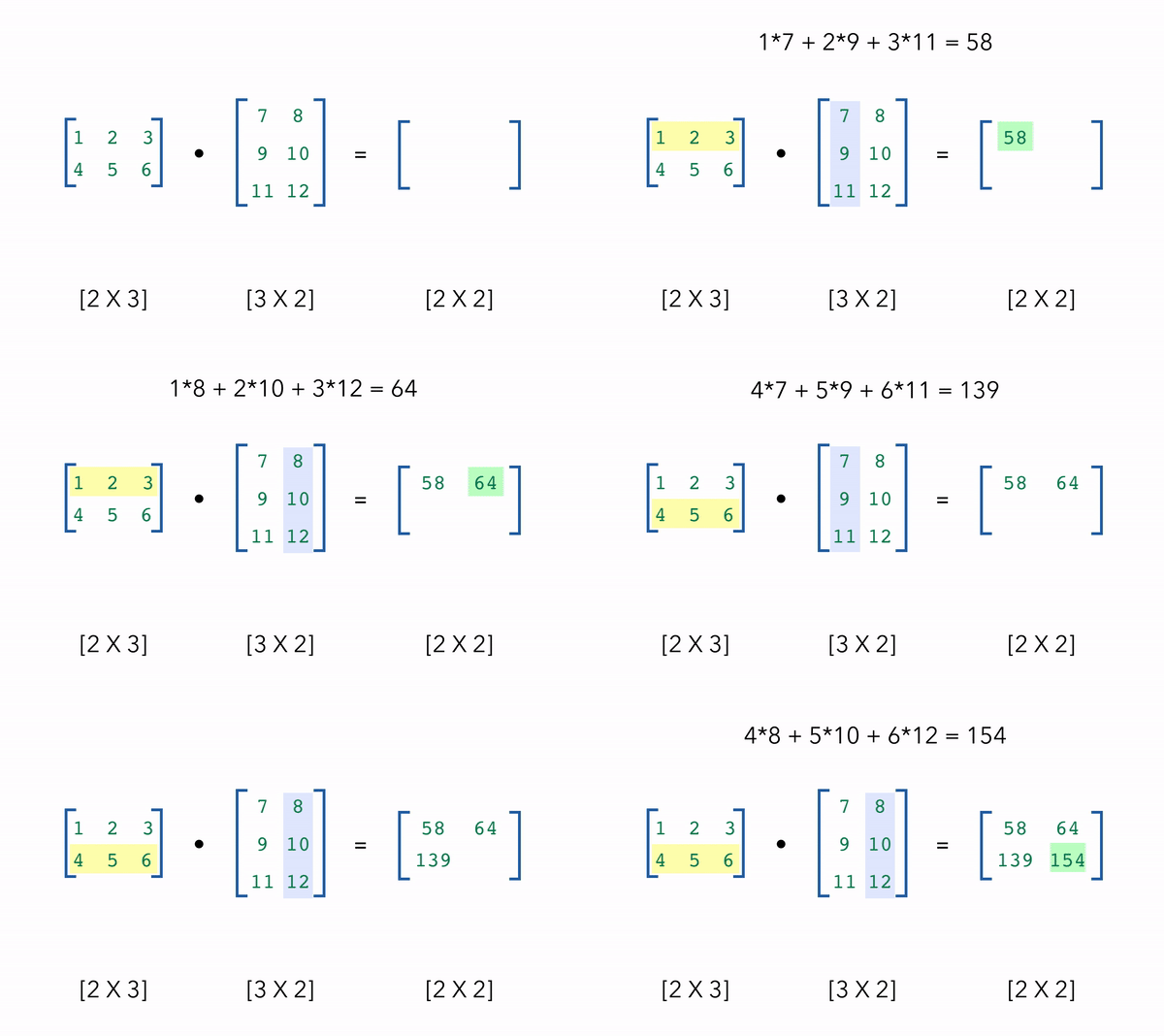
In NumPy, the modern and recommended operator for matrix multiplication is the @ symbol.

Let's see this in code.

Here is a full example of matrix-matrix multiplication:

A = np.array([[1, 2, 3],  # A is 2x3
              [4, 5, 6]])

B = np.array([[7, 8],     # B is 3x2
              [9, 10],
              [11, 12]])

# The number of columns in A (3) matches the number of rows in B (3), so we can multiply them.
# The result will have shape (rows of A, columns of B) -> (2, 2)
C = A @ B
print(f"Matrix A (2x3):\n{A}")
print(f"Matrix B (3x2):\n{B}")
print(f"Result C = A @ B (2x2):\n{C}")

Just to check the first element C[0, 0]: it's the dot product of the first row of A and the first column of B.
(1*7) + (2*9) + (3*11) = 7 + 18 + 33 = 58. This matches our result!

A = np.array([[5, 1], [3, 8]])
x = np.array([10, 1])

Conclusion

Great work on this first step into linear algebra! It might feel like a big change from data wrangling, but mastering these fundamental operations is essential for understanding what's really happening inside a machine learning model.

Key Takeaways:

• In NumPy, we represent vectors as 1D arrays and matrices as 2D arrays.
• Standard arithmetic operators (+, -, *, /) perform element-wise operations on arrays of the same shape.
• The dot product, implemented with np.dot() or the @ operator, performs linear algebraic multiplication (e.g., inner product for vectors, matrix multiplication for matrices).
• The @ operator is the modern, preferred syntax for matrix multiplication. Remember the rule: the number of columns in the first matrix must equal the number of rows in the second.

Preview of the Next Lesson:

Now that we can represent and perform basic operations on vectors and matrices, our next step is to learn how to measure their "size" or "magnitude." In the next lesson, we will learn how to compute vector and matrix norms (e.g., L1, L2, Frobenius) using NumPy. This concept is crucial for everything from regularization in regression to measuring error in model predictions.