Visualizing Data with Seaborn

1. Introduction to Seaborn

Think of Seaborn as a set of convenient functions that use Matplotlib "under the hood" to create sophisticated plots with less effort. It integrates seamlessly with Pandas DataFrames, which makes it incredibly efficient for data analysis. The standard convention for importing Seaborn is:

import seaborn as sns
import matplotlib.pyplot as plt # Often imported to customize plots further

2. Box Plots: Summarizing Distributions

A box plot (or box-and-whisker plot) provides a compact summary of a numerical variable's distribution. It's especially powerful for comparing distributions across different categories.

But to use it effectively, you first need to understand what its different parts represent.

As the video explained, a box plot shows:

• The Median (Q2): The line inside the box, representing the midpoint of the data.
• The Interquartile Range (IQR): The box itself, spanning from the 25th percentile (Q1) to the 75th percentile (Q3). The middle 50% of your data lies within this box.
• The Whiskers: The lines extending from the box, which typically represent the data range within 1.5 times the IQR. They show the overall spread of the data.
• Outliers: Individual points that fall beyond the whiskers, which are potential anomalies worth investigating.

Creating Box Plots in Seaborn

The real strength of box plots in data analysis comes from comparing distributions. With Seaborn, this is incredibly straightforward. You can compare a numerical variable across different groups defined by a categorical variable.

import seaborn as sns
import matplotlib.pyplot as plt

# Seaborn has built-in datasets. Let's use the 'tips' dataset.
tips = sns.load_dataset("tips")

# Let's look at the first few rows
print(tips.head())
#    total_bill   tip     sex smoker  day    time  size
# 0       16.99  1.01  Female     No  Sun  Dinner     2
# 1       10.34  1.66    Male     No  Sun  Dinner     3
# 2       21.01  3.50    Male     No  Sun  Dinner     3
# 3       23.68  3.31    Male     No  Sun  Dinner     2
# 4       24.59  3.61  Female     No  Sun  Dinner     4

# Create a box plot to compare total_bill across different days
plt.figure(figsize=(10, 6))
sns.boxplot(x='day', y='total_bill', data=tips)
plt.title('Distribution of Total Bill by Day')
plt.xlabel('Day of the Week')
plt.ylabel('Total Bill ($)')
plt.show()

The code above generates a plot with four box plots, one for each day, allowing for an immediate visual comparison of tipping habits.

Adding Another Layer of Comparison with hue

Seaborn makes it easy to add a second categorical variable to the comparison using the hue parameter. This splits the boxes at each x-position into multiple boxes based on the hue category, each with a different color.

The next segment of the video you watched demonstrates this perfectly, along with other practical tips.

3. Heatmaps: Visualizing Correlation Matrices

A heatmap is a graphical representation of data where the individual values contained in a matrix are represented as colors. It's a fantastic tool for finding patterns in 2D data.

In machine learning, the most common use for a heatmap is to visualize a correlation matrix. A correlation matrix shows the correlation coefficients between many pairs of variables.

• A coefficient near +1 indicates a strong positive linear relationship (as one variable increases, the other tends to increase).
• A coefficient near -1 indicates a strong negative linear relationship (as one variable increases, the other tends to decrease).
• A coefficient near 0 indicates a weak or no linear relationship.

Visualizing this matrix as a heatmap allows you to quickly spot which variables are strongly related, which is useful for tasks like feature selection.

Creating a Correlation Heatmap

The process is a simple two-step dance between Pandas and Seaborn:

1. Use the .corr() method on your DataFrame to compute the correlation matrix.
2. Pass this matrix to Seaborn's sns.heatmap() function.

The following video provides a clear, step-by-step walkthrough.

Let's put this into practice with a clear example.

Here is an example of what a finished correlation heatmap looks like. You can instantly see which variable pairs have strong relationships (brighter or darker colors) without having to scan through a table of numbers.

4. A Quick Look at Violin Plots

Before we wrap up, it's worth knowing about violin plots. A violin plot is like a combination of a box plot and a density plot (which you saw in the last lesson).

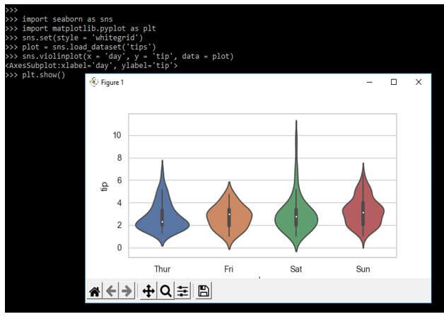
While a box plot only shows summary statistics, a violin plot also shows the full distribution of the data. This is useful because it can reveal patterns like multiple peaks (known as bimodality), which a box plot would hide. You can create one easily with sns.violinplot().

Conclusion

In this lesson, you've added two powerful statistical plots to your data visualization toolkit. You've moved beyond the basic plots in Matplotlib and have seen how Seaborn can help you create more informative graphics with minimal code.

Key Takeaways:

• Seaborn is a high-level library that simplifies the creation of complex statistical plots.
• Box plots (sns.boxplot) are excellent for summarizing a variable's distribution and are especially powerful for comparing distributions across different categories.
• Heatmaps (sns.heatmap) are the standard way to visualize correlation matrices, allowing you to quickly identify relationships between numerical variables.
• The hue parameter in Seaborn is a powerful tool for adding a second layer of categorical comparison to many plot types.

Preview of the Next Lesson:

Now that you can visualize and understand the distributions of your features, you're ready to start preparing them for machine learning models. Many algorithms perform better when numerical features are on a similar scale. In the next lesson, we will cover feature scaling, where you'll learn about StandardScaler and MinMaxScaler—two common techniques to standardize the range of your data.