Matplotlib: Basic Plotting

1. Getting Started with Matplotlib

Matplotlib is a comprehensive library for creating static, animated, and interactive visualizations in Python. The part of the library we'll use most often is pyplot, which provides a simple interface for creating plots. By convention, it's imported with the alias plt.

The basic workflow for creating a plot in Matplotlib is:

1. Prepare your data (e.g., using Python lists or Pandas Series).
2. Create a plot using a plt function (e.g., plt.plot()).
3. Customize the plot with labels, titles, colors, etc.
4. Display the plot using plt.show().

Let's start with a video that introduces Matplotlib and demonstrates this basic workflow.

2. Line Plots: Visualizing Trends

As you saw in the video, a line plot is ideal for showing how a numerical value changes over a continuous sequence, most often time. It connects a series of data points with a line, making it easy to see trends, increases, and decreases.

The core function is plt.plot(x_values, y_values).

Let's take the example from the video and add some essential customizations. A plot is not complete without clear labels and a title. These give context to the viewer.

import matplotlib.pyplot as plt

# Sample data: population (in billions) over years
year = [1950, 1970, 1990, 2010]
pop = [2.519, 3.692, 5.263, 6.972]

# 1. Create the plot
plt.plot(year, pop)

# 2. Add customizations
plt.title("World Population Growth")
plt.xlabel("Year")
plt.ylabel("Population (Billions)")

# 3. Display the plot
plt.show()

Running this code will produce a line plot with a title and labeled axes, making it much more informative. For more advanced customization, you can control the line's color, style, and markers.

# Re-plotting with style customizations
plt.plot(year, pop, color='green', marker='o', linestyle='--')

plt.title("World Population Growth")
plt.xlabel("Year")
plt.ylabel("Population (Billions)")
plt.show()

Here, color='green' sets the line color, marker='o' adds a circle at each data point, and linestyle='--' creates a dashed line.

3. Scatter Plots: Exploring Relationships

While line plots connect sequential points, scatter plots display individual data points to show the relationship between two numerical variables. They are fundamental in data exploration for machine learning, as they can help you spot correlations, clusters, and potential outliers between features.

The function for this is plt.scatter(x_values, y_values).

Let's say we have data on the heights and weights of a group of people. A scatter plot is the perfect tool to see if there's a relationship between these two measurements.

# Sample data: height (cm) and weight (kg)
height = [151, 174, 138, 186, 128, 136, 179, 163, 152, 131]
weight = [63, 81, 56, 91, 47, 57, 76, 72, 62, 48]

# Create the scatter plot
plt.scatter(height, weight)

# Add labels and title
plt.title("Height vs. Weight")
plt.xlabel("Height (cm)")
plt.ylabel("Weight (kg)")

plt.show()

You'll notice the points tend to go up and to the right, suggesting a positive correlation: taller people tend to be heavier. This is the kind of initial insight visualization provides.

A powerful technique is to use color to represent a third, categorical variable, which can reveal deeper patterns. The tutorial below demonstrates this well using the famous Iris dataset.

4. Histograms: Understanding Distributions

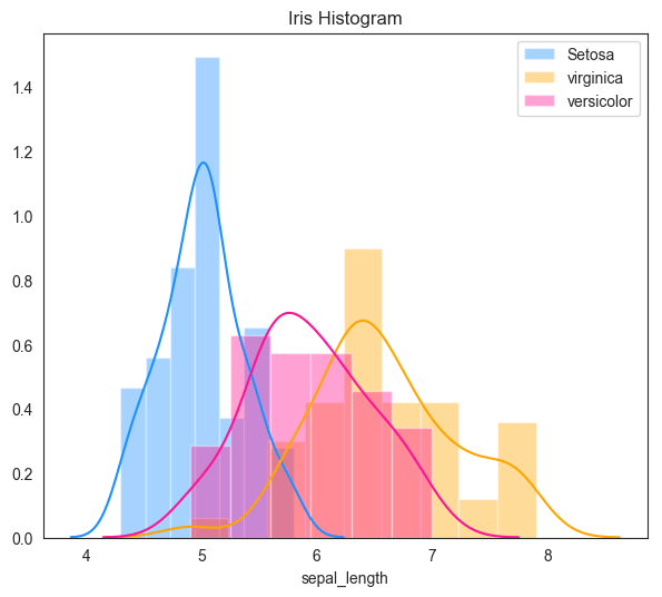
Our first two plots showed relationships between variables. A histogram, however, is used to understand the distribution of a single numerical variable. It groups numbers into ranges (called "bins") and the height of the bar shows how many data points fall into that range.

Histograms are essential for:

• Seeing the "shape" of your data (e.g., is it symmetric, skewed?).
• Identifying the central tendency (where most of the data is clustered).
• Spotting gaps or potential outliers.

In machine learning, understanding feature distributions is crucial for deciding on preprocessing steps like scaling or transformation.

The main function is plt.hist(data, bins=N), where N is the number of bins you want to divide the data into. Choosing the right number of bins is important—too few can hide patterns, and too many can create a noisy, uninformative plot.

Let's watch a video that explains histograms in detail, from the concept of bins to plotting data from a Pandas DataFrame.

As the video demonstrated, you have fine-grained control over how your data is binned. Let's create a simple histogram with a list of data.

import numpy as np

# Generate some sample data (e.g., test scores)
# np.random.randn() creates numbers from a standard normal distribution
scores = 80 + 10 * np.random.randn(1000)

# Create the histogram
plt.hist(scores, bins=30, edgecolor='black') # Using 30 bins and adding edge colors for clarity

# Add labels and title
plt.title("Distribution of Test Scores")
plt.xlabel("Score")
plt.ylabel("Frequency")

plt.show()

This plot will show you the frequency of scores across different ranges, likely revealing a "bell curve" shape, indicating that most scores are clustered around the average (80).

Conclusion

Congratulations! You've taken your first steps into the world of data visualization with Python. You now have the tools to create the three most fundamental types of plots.

Key Takeaways:

• Matplotlib (pyplot) is the foundational library for plotting in Python. The standard workflow is to plot, customize, and then show.
• Line Plots (plt.plot): Use these to visualize trends in data over a continuous interval, like time.
• Scatter Plots (plt.scatter): Use these to investigate the relationship and correlation between two numerical variables.
• Histograms (plt.hist): Use these to understand the shape, center, and spread of the distribution of a single numerical variable.

Preview of the Next Lesson:

Matplotlib is incredibly powerful but can sometimes require a lot of code for complex or aesthetically refined plots. In our next lesson, we will explore Seaborn, a high-level library built on top of Matplotlib. You'll see how Seaborn can help you create beautiful and complex statistical plots, like box plots and heatmaps, with much less code, further enhancing your ability to explore and understand your data.