Transforming Skewed Data

1. What is Skewed Data?

Skewness is a measure of the asymmetry of a probability distribution. A distribution can be symmetrical, or it can be skewed to the left or right.

• Symmetrical (No Skew): The data is evenly distributed around the mean. In a perfect normal distribution, the mean, median, and mode are all equal.
• Positive Skew (Right-Skewed): The tail on the right side of the distribution is longer. This means there are a few unusually high values. In this case, Mean > Median > Mode. This is very common in data representing quantities that can't be negative, like income, house prices, or user activity counts.
• Negative Skew (Left-Skewed): The tail on the left side is longer, indicating a few unusually low values. Here, Mean < Median < Mode.

To get a better sense of why this is important and how we can start to fix it, please watch the first couple of minutes of the following video.

In Python, using the Pandas library, you can easily calculate the skewness of a feature with the .skew() method. A common rule of thumb is:

• If skewness is between -0.5 and 0.5, the distribution is fairly symmetrical.
• If skewness is less than -0.5, the data is negatively skewed.
• If skewness is greater than 0.5, the data is positively skewed.

2. The Log Transformation for Positive Skew

The most common type of skew you'll encounter is positive skew. Fortunately, there's a very effective and widely-used technique to handle it: the logarithmic transformation.

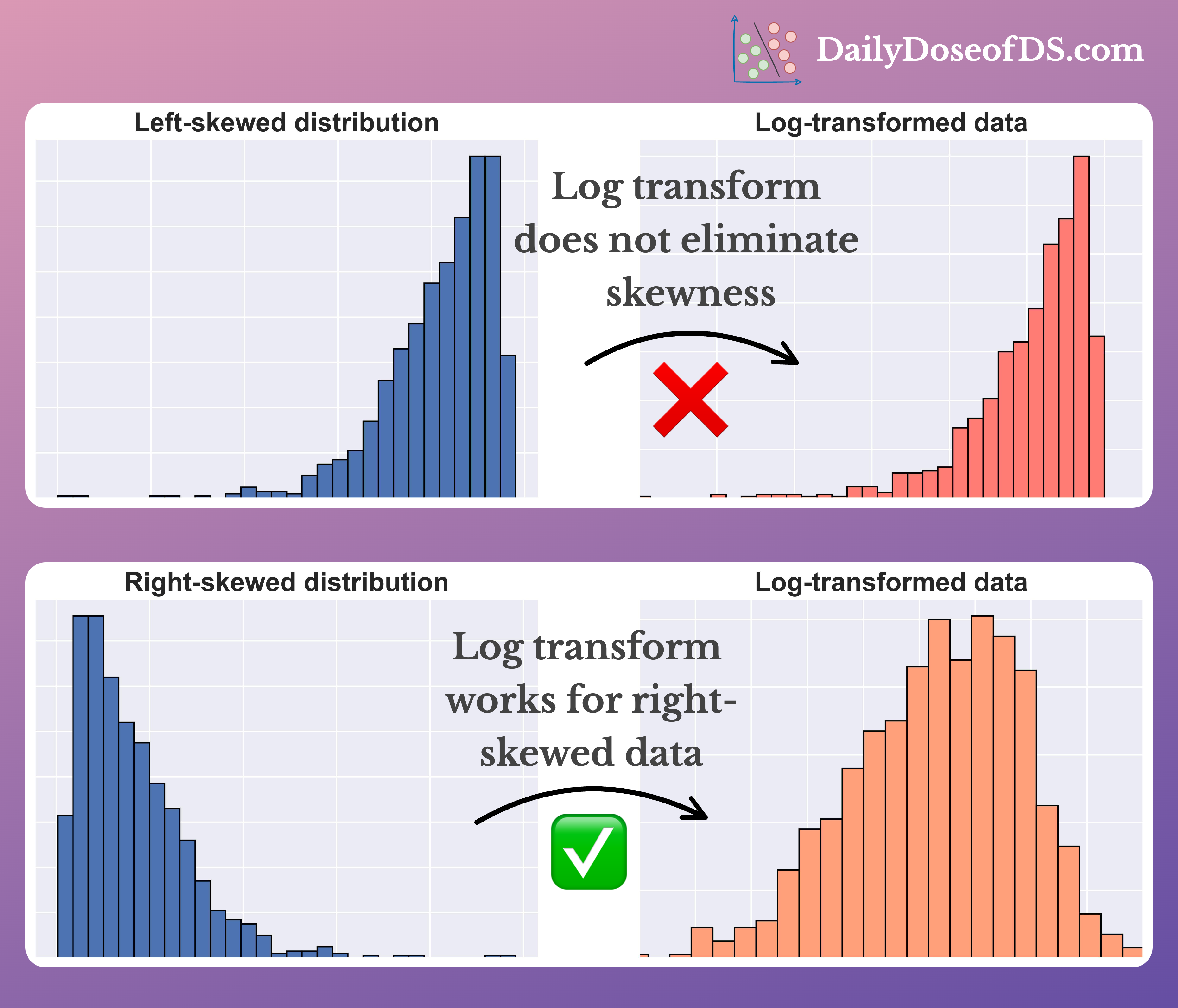
The intuition is that the logarithm function "squashes" the scale of the data. The effect is much more pronounced on large numbers than on small ones. For instance, the difference between 1000 and 100 is 900, but the difference between log(1000) and log(100) is much smaller (approx. 6.9 vs 4.6). This pulls the long right tail inwards, making the distribution more symmetrical.

A Practical Challenge: Handling Zeros

There's a catch: the logarithm function, log(x), is only defined for positive numbers (x > 0). It's undefined for zero and returns a complex number for negative values, which are not usable in most standard ML models. Since many real-world features (like "number of purchases") can contain zeros, we need a solution.

The standard workaround is the log(1+x) transformation. By adding 1 to every value before taking the log, you ensure that you are never trying to take the log of zero or a negative number (assuming your original data is non-negative). This transformation is so common that NumPy provides a dedicated function for it: np.log1p(), which computes log(1+x) with high numerical precision.

To get a solid grasp of this, let's turn to a short article that explains the log transform and its practical implementation.

Here's how you would apply this in practice with Pandas and NumPy:

import pandas as pd
import numpy as np
import seaborn as sns
import matplotlib.pyplot as plt

# 1. Create some positively skewed data
np.random.seed(0)
skewed_data = np.random.exponential(scale=200, size=1000)
df = pd.DataFrame({'feature': skewed_data})

# 2. Check the original skewness and plot
original_skew = df['feature'].skew()
print(f"Original Skewness: {original_skew:.2f}")

sns.histplot(df['feature'], kde=True)
plt.title(f"Original Distribution (Skew: {original_skew:.2f})")
plt.show()

# 3. Apply the log1p transformation
df['feature_log_transformed'] = np.log1p(df['feature'])

# 4. Check the new skewness and plot
transformed_skew = df['feature_log_transformed'].skew()
print(f"Transformed Skewness: {transformed_skew:.2f}")

sns.histplot(df['feature_log_transformed'], kde=True)
plt.title(f"Log Transformed Distribution (Skew: {transformed_skew:.2f})")
plt.show()

When you run this code, you'll see the original skewness is high (around 2.0), and the histogram has a long right tail. After the np.log1p transformation, the new skewness will be much closer to 0, and the histogram will look much more like a symmetrical bell curve.

3. A Broader View of Transformation Techniques

While the log transform is your go-to for positive skew, it's not the only tool available. Different situations might call for different methods. Let's briefly explore some other common transformations.

The following article from Machine Learning Mastery is an excellent, comprehensive guide. We will focus on the sections that introduce the different strategies.

To see some of these transformations in action, let's revisit the AnalytiCode video.

Here's a quick summary of the key alternatives:

Conclusion

You've now added another crucial technique to your data preprocessing toolkit. By identifying and correcting skewed distributions, you can satisfy the assumptions of many machine learning models and often improve their predictive performance.

Key Takeaways:

• Skewness measures the asymmetry of a feature's distribution and can negatively affect model performance.
• The most common type is positive (right) skew, where a long tail of high values pulls the mean to the right.
• The log transformation is a powerful method for correcting positive skew. Use np.log1p() to handle data that includes zeros.
• Log transforms are not suitable for data with negative values.
• For more flexibility, consider the Yeo-Johnson transformation, which works on positive, zero, and negative values, or the Box-Cox transformation for strictly positive data.
• The best transformation is often found through experimentation. Always visualize the distribution before and after to confirm its effect.

Preview of the Next Lesson:

So far, we have focused on cleaning and preparing existing features. But what if we could create entirely new features from the ones we already have? In our next lesson, we will dive into feature engineering, where you will learn how to create new features from existing data (e.g., interaction terms) to potentially unlock even better model performance.