Feature Engineering: Creating Interaction Terms

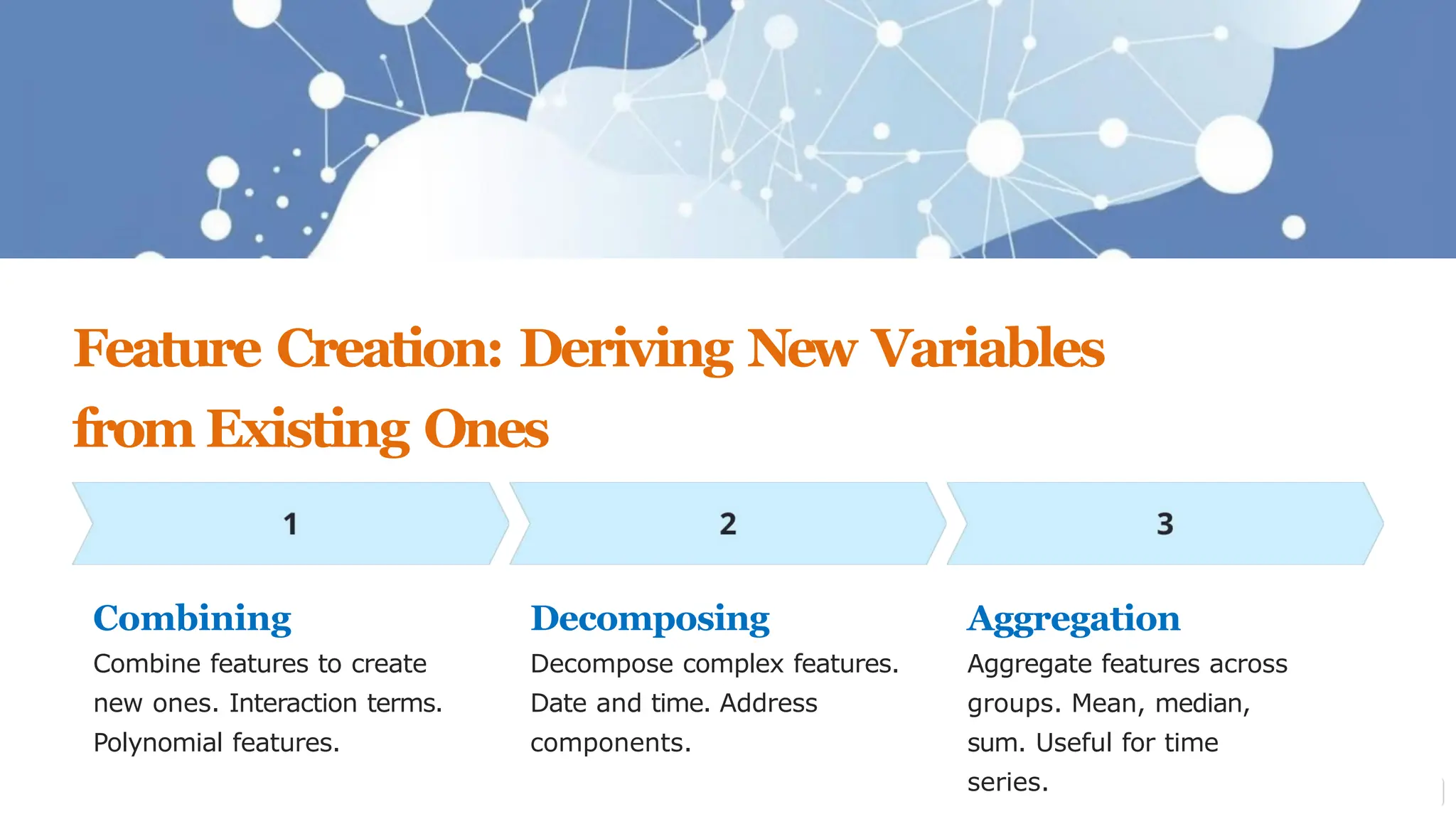
1. Creating Features with Domain Knowledge and Simple Arithmetic

Often, the most impactful new features come from a simple understanding of the data and the problem you're trying to solve. This might involve combining features with basic math (addition, subtraction, multiplication, division) to create a new variable that is more meaningful than its parts.

Let's watch a video that shows some excellent, intuitive examples of this.

As you saw in the video, these new features are often more directly related to the problem.

• FamilySize is likely more predictive of survival on the Titanic than the number of siblings and parents separately.
• TotalIncome is a more complete measure of a household's ability to repay a loan than just the applicant's income.

Here's how you can implement these ideas directly in Python using Pandas. It's often as simple as applying an arithmetic operation to existing columns.

import pandas as pd
import numpy as np

# Example 1: Creating 'TotalIncome' and 'LoanIncomeRatio'
# Let's create a sample DataFrame similar to the loan dataset
loan_data = {
    'ApplicantIncome': [5000, 6000, 3000, 4000],
    'CoapplicantIncome': [2000, 0, 1500, 5000],
    'LoanAmount': [150, 100, 100, 200]
}
df_loan = pd.DataFrame(loan_data)

# Create a 'TotalIncome' feature
df_loan['TotalIncome'] = df_loan['ApplicantIncome'] + df_loan['CoapplicantIncome']

# Create a 'LoanIncomeRatio' feature
# Adding a small constant to the denominator to avoid division by zero
df_loan['LoanIncomeRatio'] = df_loan['LoanAmount'] / (df_loan['TotalIncome'] + 1e-6)

print("Loan DataFrame with new features:")
print(df_loan)

This approach is powerful because it allows you to inject your understanding of the real world into the dataset.

2. Capturing Relationships: Interaction Terms & Polynomial Features

Sometimes, the effect of one feature depends on the value of another. For example, the positive effect of fertilizer on crop yield might only occur if there is also enough rainfall. A linear model struggles to learn this "if-then" relationship on its own.

An interaction term, created by multiplying two or more features together, makes this combined effect explicit. This allows a model to learn that fertilizer * rainfall is a potent combination.

Let's start with a video that clearly explains the "why" behind interaction features.

To formalize this and see how to implement it, we'll turn to a textual resource and scikit-learn's PolynomialFeatures transformer. This powerful tool can create both interaction terms and polynomial features (e.g., $x^2$, $x^3$), which help models capture curved, non-linear relationships.

Now that you have the theory, let's see PolynomialFeatures in action.

Here's a summary of the implementation in Python. Notice how we can control whether we get only interactions or full polynomial features.

from sklearn.preprocessing import PolynomialFeatures

# Sample data with two features
X = np.array([[2, 3],
              [4, 5],
              [6, 7]])
features_df = pd.DataFrame(X, columns=['x1', 'x2'])
print("Original Features:")
print(features_df)

# 1. Interaction terms only
# This creates the original features plus the interaction term (x1 * x2)
poly_interact = PolynomialFeatures(degree=2, interaction_only=True, include_bias=False)
X_interact = poly_interact.fit_transform(X)

# Get feature names for clarity
interact_names = poly_interact.get_feature_names_out(['x1', 'x2'])
interact_df = pd.DataFrame(X_interact, columns=interact_names)

print("\nFeatures with Interactions Only:")
print(interact_df)


# 2. Full polynomial features (degree 2)
# This creates original features, interaction term (x1*x2), and squared terms (x1^2, x2^2)
poly_full = PolynomialFeatures(degree=2, interaction_only=False, include_bias=False)
X_full = poly_full.fit_transform(X)

# Get feature names for clarity
full_names = poly_full.get_feature_names_out(['x1', 'x2'])
full_df = pd.DataFrame(X_full, columns=full_names)

print("\nFeatures with Full Polynomials (degree=2):")
print(full_df)

A key takeaway is that while these features can be very powerful, they also increase the complexity of your model and the risk of overfitting. It's crucial to start with a low degree (like 2) and be mindful of the number of features you're creating.

3. Decomposing Complex Features: The Case of Datetime

Some features, like a timestamp, contain a wealth of information packed into a single column. "Decomposing" such a feature means breaking it down into its constituent parts, each becoming a new feature.

A timestamp like 2023-10-27 15:30:00 can tell you:

• Year: 2023
• Month: 10 (October)
• Day of month: 27
• Day of week: 4 (Friday)
• Hour: 15 (3 PM)
• Is it a weekend? No.
• Is it the end of the month? Yes.

Each of these could be a valuable signal for a machine learning model. Pandas makes this decomposition incredibly easy using the .dt accessor.

Let's put that into a clean code example. The key is to first ensure your column is in a proper datetime format using pd.to_datetime().

# Create a sample DataFrame with date strings
date_data = {'event_time': ['2023-01-15 08:30:00', '2023-07-22 21:00:00', '2024-12-25 12:00:00']}
df_dates = pd.DataFrame(date_data)

# 1. Convert the column to datetime objects
df_dates['event_time'] = pd.to_datetime(df_dates['event_time'])
print("Original DataFrame with correct dtype:")
print(df_dates.info())

# 2. Decompose the datetime into new features
df_dates['year'] = df_dates['event_time'].dt.year
df_dates['month'] = df_dates['event_time'].dt.month
df_dates['day_of_week'] = df_dates['event_time'].dt.dayofweek # Monday=0, Sunday=6
df_dates['hour'] = df_dates['event_time'].dt.hour
df_dates['is_weekend'] = df_dates['event_time'].dt.dayofweek.isin([5, 6]).astype(int)

print("\nDataFrame with new datetime features:")
print(df_dates)

Conclusion

Congratulations! You've just learned the fundamentals of feature engineering, a skill that separates good machine learning practitioners from great ones. You now have a range of techniques to create new, potentially powerful features from the data you already have.

Key Takeaways:

• Feature Engineering is the process of creating new features to improve model performance. It's as much an art as it is a science.
• New features can be created through:
  • Domain Knowledge: Using simple arithmetic (+, -, *, /) to combine features in a way that makes real-world sense (e.g., TotalIncome).
  • Interaction Terms: Multiplying features to help linear models capture combined effects (e.g., temperature * humidity). PolynomialFeatures is the tool for this.
  • Decomposition: Breaking down complex features like datetimes into simpler parts (e.g., year, month, hour) using tools like Pandas' .dt accessor.

Preview of the Next Lesson:

We've now covered all the key individual steps of data preparation: scaling, encoding, transforming, and creating features. But how do you put them all together in an organized, efficient, and reproducible way? In our next lesson, you will learn how to build a data preprocessing pipeline using scikit-learn's Pipeline and ColumnTransformer. This is the final step in creating a professional machine learning workflow.