Hello! Welcome back to our journey into Supervised Learning.
In our last lesson, we built a simple linear regression model from the ground up. You saw how the Ordinary Least Squares (OLS) method uses calculus to derive direct formulas for the slope and intercept, allowing us to fit a line to data with a single input feature. This was a crucial first step, but most real-world problems aren't that simple.
This lesson builds directly on that foundation. We will extend linear regression to handle multiple features, a technique known as Multiple Linear Regression (MLR). Instead of just predicting a house's price from its size, we'll see how to build a model that considers size, age, number of bedrooms, and more, all at once. This will make our models significantly more powerful and realistic. We will explore the new mathematical form this takes and see how to solve it both analytically and through iterative methods.
1. From a Line to a Hyperplane
In simple linear regression, our model was a line described by the equation:
Here, is the intercept and is the coefficient (slope) for our single feature, .
To incorporate more features, we simply extend this equation by adding more terms, one for each new feature:
- is still our predicted value.
- are the different features.
- is the intercept.
- are the coefficients for each feature. Each represents the change in for a one-unit change in , assuming all other features are held constant.
Visually, we're no longer fitting a 2D line. With two features (), we're fitting a 3D plane. With more than two features, we're fitting a hyperplane, which is just the general term for a flat surface in a multi-dimensional space.
To get a clearer picture of this transition, please start by reading the first two short sections of the following guide.
Multiple Linear Regression: Complete Guide with Formulas ...
This article, 'Multiple Linear Regression: Complete Guide', introduces the core concept of MLR and how it extends simple linear regression by fitting a hyperplane.
Please read the introductory section titled 'Multiple Linear Regression'. Focus on the key insight that real-world outcomes are influenced by multiple factors simultaneously.
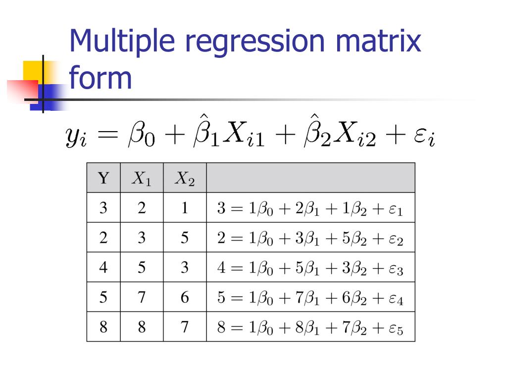
2. The Power of Matrix Notation
As you can see, the equation gets long and clumsy with many features. Your computer science background will appreciate that we can represent this much more elegantly using linear algebra.
The entire system of equations for all our data points can be expressed in a single, compact form:
Let's break down each component:
- is a vector containing the actual target values for all observations in our dataset.
- is a vector containing all our model's coefficients ().
- is a vector containing the error terms (residuals) for each observation.
- is the design matrix. This is a crucial concept. It's an matrix where each row is an observation and each column is a feature. We add a special first column of all ones. This "dummy" column corresponds to the intercept term , ensuring it gets estimated correctly.
The video below provides an excellent visual breakdown of how the individual data points are organized into these vectors and the design matrix.
Matrix Form Multiple Linear Regression MLR
This video, 'Matrix Form Multiple Linear Regression', clearly demonstrates how the familiar scalar equation is converted into the compact matrix form. It's a great way to visualize the structure of the y vector, the β vector, and especially the design matrix X.
Watch the video from the beginning until 08:40. Pay close attention to: The structure of the y vector (dependent variables). The structure of the design matrix X, particularly the column of ones for the intercept. The structure of the β vector (coefficients). How the dimensions of these matrices (n, p+1) must align for multiplication.
Test your understanding!
Suppose you have the following small dataset to predict house price (y) from size (x1) and number of bedrooms (x2).
| Price (y) | Size (x1) | Bedrooms (x2) |
|---|---|---|
| 300 | 1500 | 3 |
| 450 | 2000 | 4 |
What would the design matrix X and the coefficient vector β look like in their general form for this problem?
Show answer
The design matrix X would have 2 rows (for the 2 houses) and 3 columns (for the intercept, size, and bedrooms).
The coefficient vector β would have 3 elements, one for the intercept and one for each feature.
3. Finding the Optimal Coefficients
Just like in simple linear regression, our goal is to find the coefficient vector that minimizes the sum of squared errors (SSE).
In matrix form, this is written as:
There are two primary methods to find the that minimizes this SSE.
Method 1: The Normal Equation (Analytical Solution)
This is the multi-feature equivalent of the OLS formulas we derived in the last lesson. By using matrix calculus to take the derivative of the SSE with respect to and setting it to zero, we arrive at a beautiful closed-form solution called the Normal Equation:
- is our estimated coefficient vector.
- is the transpose of the design matrix .
- is the inverse of the matrix product .
This equation gives us the exact optimal coefficients in one direct calculation!
To see how this equation is derived and used, continue with the video from Boer Commander.
Matrix Form Multiple Linear Regression MLR
The video now connects the minimization of the SSE to the Normal Equation, showing that this formula is the direct solution.
Watch the segment from 08:40 to 12:11. The key takeaway is that the formula β_hat = (X'X)^-1 * X'Y is the result of minimizing the sum of squared errors, just for multiple features.
The main advantage of the Normal Equation is its directness. However, calculating the matrix inverse is computationally very expensive, especially for datasets with a large number of features. Its complexity is roughly , where is the number of features. This makes it impractical for problems with tens of thousands of features.
Method 2: Gradient Descent (Iterative Solution)
When the Normal Equation is too slow, we turn to gradient descent. As you'll recall from our Calculus module, this is an iterative optimization algorithm that finds the minimum of a function.
The process is:
- Start with some initial values for the coefficients in (e.g., all zeros).
- Calculate the cost (SSE) for the current coefficients.
- Calculate the gradient (the partial derivative of the cost function with respect to each coefficient). This tells us the direction of steepest ascent.
- Update each coefficient by taking a small step in the opposite direction of the gradient. The size of this step is controlled by the learning rate, .
- Repeat steps 2-4 until the cost function converges to a minimum.
The update rule for each coefficient in the vector is:
where is our cost function.
The following video provides an excellent and in-depth explanation of linear regression with multiple features and how gradient descent is used to optimize the parameters.
Stanford CS229: Machine Learning - Linear Regression and Gradient Descent | Lecture 2 (Autumn 2018)
In this classic lecture from Stanford's CS229 course, Andrew Ng explains the formulation of multiple linear regression and the gradient descent algorithm.
Please watch from 01:46 to 34:16. Focus on these key concepts: Hypothesis Representation (01:46 - 12:36): How the hypothesis function is extended for multiple features and the introduction of the x_0=1 dummy feature. Cost Function (12:46 - 17:52): Understanding the mean squared error cost function for multiple parameters. Gradient Descent (17:52 - 34:16): The core of the algorithm. Pay attention to the update rule and the derivation of the partial derivative term. Don't worry if the calculus is a bit fast; the main idea is to understand the iterative update process.
In practice, for very large datasets, a variant called Stochastic Gradient Descent (SGD) is often used. Instead of calculating the gradient using the entire dataset in each step (which is slow), SGD updates the parameters using just one training example at a time. This makes progress much faster, though the path to the minimum is "noisier." The Stanford video mentions this toward the end (starting at 44:19), which you can explore if you're curious, but it's not essential for this lesson.
4. Implementation in Python
Now, let's put this theory into code. We'll use the excellent guide from mbrenndoerfer.com to see how to implement MLR.
First, we'll see how to do it with scikit-learn, which is the standard practical approach. Then, for a deeper understanding, we will implement the Normal Equation from scratch using NumPy.
Multiple Linear Regression: Complete Guide with Formulas ...
This guide provides a fantastic, clear walkthrough of implementing multiple linear regression in Python. We'll focus on the implementation section.
Read the section titled 'Implementation'. Follow the steps carefully: Step 1 & 2: See how to fit a model and make predictions using scikit-learn. Notice how simple it is. Step 3: This is the most important part for our learning. Study the multiple_linear_regression function that implements the Normal Equation (X'X)^(-1)X'Y using NumPy. Note the use of np.linalg.solve() for better numerical stability than calculating the inverse directly. Step 4: Skim through the real-world example to see how these concepts apply to a larger, more realistic dataset.
Here's the key code block from that article for implementing the Normal Equation with NumPy. It's a direct translation of the math into code.
import numpy as np

def multiple_linear_regression_normal_equation(X, y):
    """
    Fits multiple linear regression using the closed-form OLS solution (Normal Equation).

    Parameters:
    X: Feature matrix (n_samples, n_features)
    y: Target vector (n_samples,)

    Returns:
    coefficients: Array of coefficients [intercept, feature1, feature2, ...]
    """
    # Add a column of ones to X for the intercept term
    X_with_intercept = np.c_[np.ones(X.shape[0]), X]

    # Compute the OLS solution: β = (X'X)^(-1) X'y
    XtX = X_with_intercept.T @ X_with_intercept
    Xty = X_with_intercept.T @ y

    # Use np.linalg.solve for better numerical stability and efficiency
    # This solves the equation XtX * β = Xty for β
    coefficients = np.linalg.solve(XtX, Xty)

    return coefficients

# --- Let's test it on a small dataset ---
# Features: [size in sq ft, age in years]
X_np = np.array([[2000, 1], [1500, 5], [2500, 2]])
# Target: price in thousands
y_np = np.array([400, 300, 500])

# Get the coefficients
coeffs = multiple_linear_regression_normal_equation(X_np, y_np)
intercept, slope_size, slope_age = coeffs[0], coeffs[1], coeffs[2]

print(f"Calculated coefficients using Normal Equation:")
print(f"Intercept (β0): {intercept:.4f}")
print(f"Size coefficient (β1): {slope_size:.4f}")
print(f"Age coefficient (β2): {slope_age:.4f}")

# Compare with scikit-learn
from sklearn.linear_model import LinearRegression

model = LinearRegression()
model.fit(X_np, y_np)

print("\nScikit-learn's coefficients:")
print(f"Intercept (β0): {model.intercept_:.4f}")
print(f"Coefficients (β1, β2): {model.coef_}")
Running this code confirms that our from-scratch implementation of the Normal Equation yields the same results as scikit-learn, proving our understanding of the underlying mechanics.
Conclusion
In this lesson, you've made a significant leap from simple to multiple linear regression, unlocking the ability to model more complex, real-world relationships.
Key Takeaways:
- Multiple Linear Regression extends the simple model by adding a coefficient for each additional feature, fitting a hyperplane to the data.
- The equation can be expressed compactly using matrix notation: . The design matrix , with its leading column of ones, is a key component.
- There are two main ways to find the optimal coefficients that minimize SSE:
- The Normal Equation: A direct, analytical solution that is elegant but computationally expensive for many features.
- Gradient Descent: An iterative optimization approach that is more scalable and widely used in modern machine learning.
Preview of the Next Lesson:
You might think linear regression can only model linear relationships, but that's not quite true! In our next lesson, we will explore Polynomial Regression. You'll learn a clever technique to use the linear regression framework we've just studied to fit non-linear, curved data by creating new features from our existing ones.