Hello! Let's dive into the next topic in our regression module.
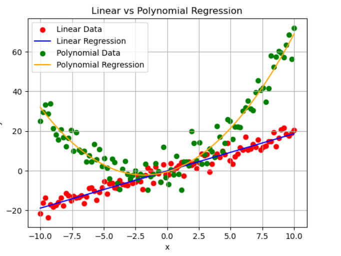
In our last lesson, we saw how to extend linear regression to handle multiple features, allowing us to model relationships like a house's price based on its size, age, and location. Our models, however, were always "flat"—lines, planes, or hyperplanes. But what happens when the relationship between variables isn't linear? What if it's curved?
This lesson will equip you with a powerful technique to handle exactly that. We'll explore Polynomial Regression, a method that cleverly uses the linear regression machinery you've already mastered to model non-linear, curved data. You'll learn how to create new features from existing ones to capture these curves, a process that is a cornerstone of machine learning called feature engineering.
By the end of this lesson, you will be able to apply polynomial regression to model these non-linear relationships and understand the critical trade-off between model complexity and the risk of overfitting.
1. The Core Idea: Bending the Line with Feature Engineering
At first, it might seem contradictory: how can we use a linear model to fit a non-linear curve? The secret is that we don't change the linear regression algorithm at all. Instead, we transform our features.
Imagine you have a single feature, . Simple linear regression tries to find the best fit for the model:
To model a curve, we can create new features by taking our original feature to higher powers, like , , etc. Then, we fit a linear regression model to this expanded set of features. For a degree-2 polynomial, our model becomes:
From the model's perspective, this is just a multiple linear regression problem with two features: and . The model is still linear with respect to its coefficients (), which is the key property that allows us to use all the same solvers, like the Normal Equation or Gradient Descent.
To solidify this crucial concept, the following video explains what a polynomial is and why polynomial regression is still considered a general linear model.
In this video, 'Polynomial regression' by Mike X Cohen, the presenter clarifies the definition of a polynomial and explains why this method, despite capturing non-linear data patterns, is fundamentally a linear model.
Watch from the beginning to 05:35. Focus on: The definition of a polynomial and its 'order' (or degree). The key insight that the model remains linear because the coefficients (the β values) are not transformed. The visual examples of data patterns where a polynomial model is more appropriate than a simple line.
This process of creating new features from existing ones is often called basis expansion. It's a fundamental concept in machine learning for increasing a model's complexity and flexibility.
2. Implementing Polynomial Regression in Python
In practice, you don't need to manually calculate the squared and cubed terms. Scikit-learn provides a convenient transformer called PolynomialFeatures to do this for you.
The workflow is a two-step process:
- Transform your data: Use
PolynomialFeaturesto generate a new feature matrix that includes the original feature, its higher-degree powers, and (if you have multiple features) their interaction terms. - Fit a linear model: Use a standard
LinearRegressionmodel on the new, transformed feature matrix.
The video below demonstrates this process in Python. It starts by showing how linear regression fails on curved data and then introduces PolynomialFeatures as the solution.
Polynomial Regression in Python
This video, 'Polynomial Regression in Python' from NeuralNine, provides a practical, code-first demonstration of the concepts we've just discussed.
Watch from the beginning to 12:30. Pay attention to: The initial example showing why linear regression is insufficient for quadratic data (up to 10:47). How to use PolynomialFeatures to transform the input features (from 10:47 onwards).
Using a Pipeline for a Cleaner Workflow
Chaining the PolynomialFeatures transformer and the LinearRegression estimator together can be made more robust and streamlined using a Pipeline. A pipeline bundles these steps into a single object that behaves like a standard scikit-learn model. This is the recommended best practice as it prevents mistakes, such as forgetting to apply the same transformation to your test data.
The following guide walks through a complete implementation, from generating synthetic data to building and evaluating a model using a Pipeline.
Polynomial Regression: Complete Guide with Math ...
This guide, 'Polynomial Regression: Complete Guide with Math ...' provides a thorough walkthrough of implementing polynomial regression in scikit-learn. We'll focus on the coding part.
Please read the sections titled 'Implementation in Scikit-learn' and 'Key Parameters'. Focus on the following: Setting Up the Data: How synthetic non-linear data is generated. Building a Polynomial Regression Pipeline: Understand how PolynomialFeatures and LinearRegression are combined into a single Pipeline object. Key Parameters: Pay special attention to the degree parameter in PolynomialFeatures, as it's the most important hyperparameter you'll tune.
Here is a typical code structure for a polynomial regression pipeline:
import numpy as np
from sklearn.preprocessing import PolynomialFeatures
from sklearn.linear_model import LinearRegression
from sklearn.pipeline import Pipeline

# 1. Generate some non-linear data
X = np.linspace(-5, 5, 100).reshape(-1, 1)
y = 0.5 * X**2 + X + 2 + np.random.randn(100, 1)

# 2. Create a pipeline
# The degree parameter controls the complexity of the model.
polynomial_degree = 2

poly_reg_pipeline = Pipeline([
    ("poly_features", PolynomialFeatures(degree=polynomial_degree, include_bias=False)),
    ("linear_reg", LinearRegression())
])

# 3. Fit the model
poly_reg_pipeline.fit(X, y)

# 4. Make predictions
# The pipeline automatically handles the feature transformation for new data.
y_pred = poly_reg_pipeline.predict(X)

print(f"Model trained for degree {polynomial_degree}.")
3. The Danger: Overfitting and the Bias-Variance Trade-off
Polynomial regression is powerful, but that power comes with a risk. The degree parameter is a double-edged sword.
- Low degree (e.g., 1): The model is too simple and cannot capture the curve in the data. This is called underfitting (high bias, low variance).
- High degree (e.g., 20): The model is extremely flexible and can wiggle its way through every single data point, including the random noise. It will have a near-perfect score on the training data but will fail miserably on new, unseen data. This is called overfitting (low bias, high variance).
- Just right degree: The model captures the underlying trend without fitting the noise. This is the goal.
This is a classic example of the bias-variance trade-off, a central concept in machine learning that we discussed in Module 9.
The video you watched earlier contains excellent segments that illustrate this exact problem.
Polynomial Regression in Python
Let's return to the NeuralNine video to see a visual demonstration of overfitting.
Watch the segment from 12:30 to 14:39 to understand the conceptual danger of high degrees. Then, watch from 16:32 to 19:42 to see clear examples of how increasing the degree and noise leads to wild, overfitted curves.
Choosing the right degree is a process of model selection. A common approach is to train models with different degrees and evaluate their performance on a separate validation set. You choose the degree that gives the best performance on the validation data, not the training data.
Test your understanding!
Look at the three plots below showing models of different polynomial degrees fit to the same dataset.
- Plot A: A straight line that misses the curve in the data.
- Plot B: A very complex curve that passes through almost every data point.
- Plot C: A smooth curve that captures the general trend of the data.
Which plot represents underfitting, which represents overfitting, and which is likely the best model?
Show answer
- Plot A represents underfitting. The model is too simple (likely degree=1) and has high bias.
- Plot B represents overfitting. The model is too complex (a very high degree) and is fitting the noise in the training data. It has high variance.
- Plot C represents a good fit. It has found a good balance between bias and variance.
Conclusion
In this lesson, you've learned how to break the "linear" barrier of linear regression to model complex, curved relationships.
Key Takeaways:
- Polynomial Regression is a form of linear regression that uses features transformed into their polynomial powers (e.g., ).
- It is a type of feature engineering or basis expansion that increases model flexibility.
- The model is still linear with respect to its coefficients, which allows us to use standard OLS solvers.
- In
scikit-learn, this is implemented usingPolynomialFeaturesandLinearRegression, ideally combined within aPipeline. - The
degreeparameter controls model complexity, and choosing a degree that is too high leads to overfitting.
Preview of the Next Lesson:
We've seen that high-degree polynomial models are prone to overfitting because their coefficients can become very large, leading to wild functions. But what if the underlying relationship is truly complex and requires a high-degree model? Is there a way to use a complex model without it overfitting? The answer is yes. In our next lesson, we will explore Regularization. You will learn about Ridge and Lasso regression, two powerful techniques that constrain the model's coefficients to prevent them from getting too large, allowing us to build complex yet robust models.