Hello! Welcome to your next lesson in the Introduction to Machine Learning module.
In our last lesson, we covered the essential metrics for evaluating model performance, such as Mean Squared Error for regression and Precision/Recall for classification. We learned what to measure to determine if a model is performing well.
Today, we'll build on that by learning how to use those metrics to diagnose two of the most fundamental challenges in machine learning: underfitting and overfitting. This is a critical skill for any machine learning practitioner. By the end of this lesson, you will be able to diagnose these issues by comparing a model's performance on the data it was trained on versus new, unseen data.
Introduction: The Goal of Generalization
The ultimate goal of a machine learning model is not just to perform well on the data it has already seen, but to generalize its learning to make accurate predictions on new, unseen data.
- Underfitting occurs when a model is too simple to capture the underlying patterns in the training data. It performs poorly on both the training data and new data. Think of it as a student who didn't study enough for an exam and fails both the practice questions and the final test.
- Overfitting occurs when a model learns the training data too well, including its noise and random fluctuations. It performs exceptionally well on the training data but fails to generalize to new data. This is like a student who memorizes the answers to the practice questions but doesn't understand the concepts, so they fail the final test which has different questions.
Our main diagnostic tool will be to compare the model's performance on the training set against its performance on the validation set.
1. Building the Core Concepts
To start, let's build an intuitive understanding of overfitting and underfitting. The best way to do this is with an analogy and some clear visual examples.
A Critical Skill People Learn Too LATE: Learning Curves In Machine Learning.
This video from the Underfitted channel uses a great student-teacher analogy to introduce overfitting and underfitting. It clearly explains why we want models that generalize their knowledge.
Watch the first two minutes of the video (00:00 - 02:01) to grasp the core analogy and the definitions of overfitting and underfitting.
Now, let's connect this idea to what happens mathematically. A common way to visualize this is by looking at how the complexity of a model affects its ability to fit the data.
This image shows the relationship between model complexity and error.
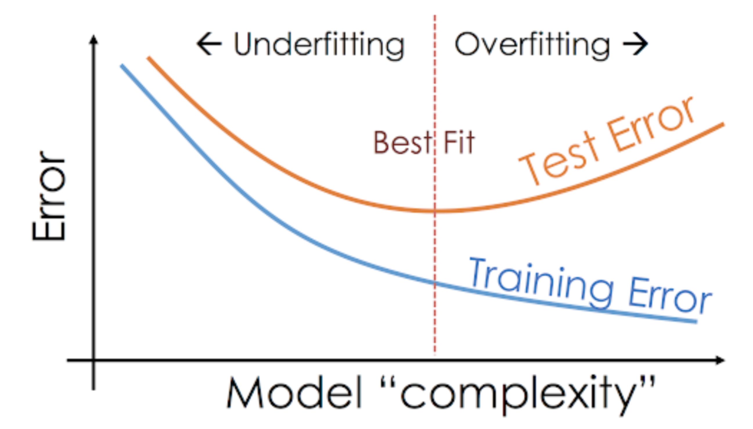
As you can see, a model that is too simple (low complexity) is underfit. A model that is too complex is overfit. Our goal is to find that "sweet spot" in the middle.
Let's see a practical example of this using polynomial regression, which should be a familiar concept from your math studies.
Machine Learning-Bias And Variance In Depth Intuition| Overfitting Underfitting
Krish Naik provides an excellent visual intuition for this concept. He shows how increasing the degree of a polynomial regression model can lead it from being underfit to well-fit, and finally to overfit.
Watch the segment from 00:36 to 04:54. Focus on: How a low-degree polynomial (a straight line) fails to capture the curve (underfitting). How a very high-degree polynomial fits every single training point perfectly but would likely perform poorly on new points (overfitting). The distinction between performance on training data versus test data.
2. Using Learning Curves for Diagnosis
The most powerful tool for diagnosing overfitting and underfitting is the learning curve. A learning curve plots a performance metric (like error or accuracy) against the amount of experience (e.g., training iterations, or epochs). We plot two curves on the same graph: one for the training set and one for the validation set. The relationship between these two curves tells us what's happening with our model.
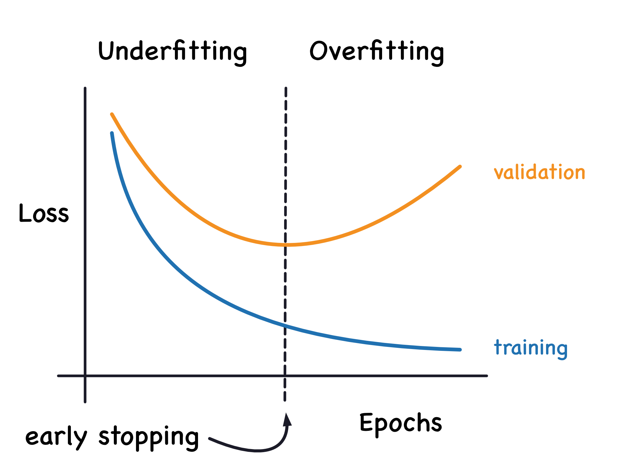
Let's dive deeper into how to interpret these curves.
A Critical Skill People Learn Too LATE: Learning Curves In Machine Learning.
Let's return to the Underfitted video, which provides a masterclass in reading learning curves.
Watch the rest of the video from 02:01 to 06:12. Pay close attention to the visual characteristics of the curves for each scenario: Underfitting: What does it look like when the training loss is high? Overfitting: What is the key sign when you compare the training loss and the testing loss? Well-fit: What do the ideal curves look like? Special Cases: Notice the two common patterns: a large gap between the curves, and the validation loss increasing after a certain point.
To solidify your understanding and see how this is implemented in Python, the following article provides a great summary with code.
Learning Curve To Identify Overfit & Underfit
This GeeksforGeeks article provides clear definitions and code examples for generating learning curves for well-fit, overfit, and underfit models.
Read the sections 'Identifying Overfitting and Underfitting Using Learning Curves', 'Learning Curve of an Overfit Model', and 'Learning Curve of an Underfit Model'. Focus on connecting the descriptions of the curves back to the visuals you just saw in the video: Overfit: Notice the "significant gap" between the continuously decreasing training error and the validation error that stops improving or gets worse. Underfit: Notice that both training and validation errors are high and plateau close to each other.
3. Practical Diagnosis by Comparing Performance Metrics
While learning curves are visually powerful, the core of the diagnosis comes down to a simple comparison of performance metrics. You've already learned about metrics like Mean Squared Error (MSE). Let's see how to use them directly.
The process is straightforward:
- Train your model on the training data.
- Calculate the error (e.g., MSE) on the training data.
- Calculate the error on the validation/test data.
- Compare the two error values.
This next resource provides a concise, hands-on tutorial for doing exactly this.
Diagnosing and Fixing Overfitting in Machine Learning with Python
This Machine Learning Mastery article demonstrates how to intentionally create an overfit model and diagnose it by comparing the training and test MSE. This is a very practical, code-first approach.
Read the section titled 'Diagnosing Overfitting'. The code defines a function that trains a polynomial regression model. Follow the example where overfit_degree = 10 is used. The key insight is in the final print statement, which shows the Train MSE and Test MSE. Observe the massive difference between them—this is the classic signature of overfitting.
As you saw in the article, the overfit model had a tiny training MSE (0.0052) but an enormous test MSE (406.1920). This huge gap is your red flag for overfitting.
- Low Training Error + High Validation Error = Overfitting.
- High Training Error + High Validation Error = Underfitting.
- Low Training Error + Low Validation Error = Good Fit!
Test your understanding!
You are working on a house price prediction project (a regression task). You have trained three different models and evaluated their Root Mean Squared Error (RMSE) on both the training and validation sets.
- Model A:
- Training RMSE: $55,000
- Validation RMSE: $58,000
- Model B:
- Training RMSE: $5,000
- Validation RMSE: $60,000
- Model C:
- Training RMSE: $95,000
- Validation RMSE: $98,000
Which model is overfitting, which is underfitting, and which seems to be the best fit? Explain your reasoning.
Show answer
-
Model B is overfitting. It has an extremely low error on the training data ($5,000) but a very high error on the validation data ($60,000). The huge gap between the two indicates that the model has memorized the training data and cannot generalize.
-
Model C is underfitting. It performs poorly on both the training data ($95,000) and the validation data ($98,000). The high error on the training set itself shows that the model is too simple to capture the underlying patterns in the data.
-
Model A is the best fit. It has a reasonably low error on both the training ($55,000) and validation ($58,000) sets. Crucially, the performance is very similar on both, indicating that it is generalizing well.
Conclusion
Congratulations! You can now diagnose two of the most common failure modes in machine learning. By understanding how to spot overfitting and underfitting, you have moved from simply building models to being able to debug and improve them.
Key Takeaways:
- Generalization is the primary goal: a model should perform well on new, unseen data.
- Underfitting (high bias) means the model is too simple. It is characterized by high error on both the training and validation sets. The learning curves will plateau at a high error level.
- Overfitting (high variance) means the model is too complex and has memorized the training data. It is characterized by low error on the training set but high error on the validation set. The learning curves will show a significant and growing gap between the training and validation error.
- A well-fit model shows low error on both the training and validation sets, with a small gap between the two.
Preview of the Next Lesson:
We've learned how to identify overfitting and underfitting. The next logical question is: how do we fix them? In our next lesson, we will explore common strategies to mitigate these problems, such as changing model complexity, using regularization, and gathering more data.