Vanishing and Exploding Gradients in Vanilla RNNs

Hello! This course begins with a time-sensitive sequence-modeling sprint, alongside the longer systems and C++ track. In this first lesson, you will build the mathematical picture needed for that sprint: how a vanilla recurrent neural network (RNN) updates its state, and why training it on a long stream can become difficult even when the forward computation is straightforward.

By the end, you should be able to write the recurrence with correctly shaped matrices, trace how an early input can affect a later prediction, and identify the repeated derivatives responsible for vanishing or exploding gradients. Allow about 40 minutes, including the video and reading below.

One update rule, reused over time

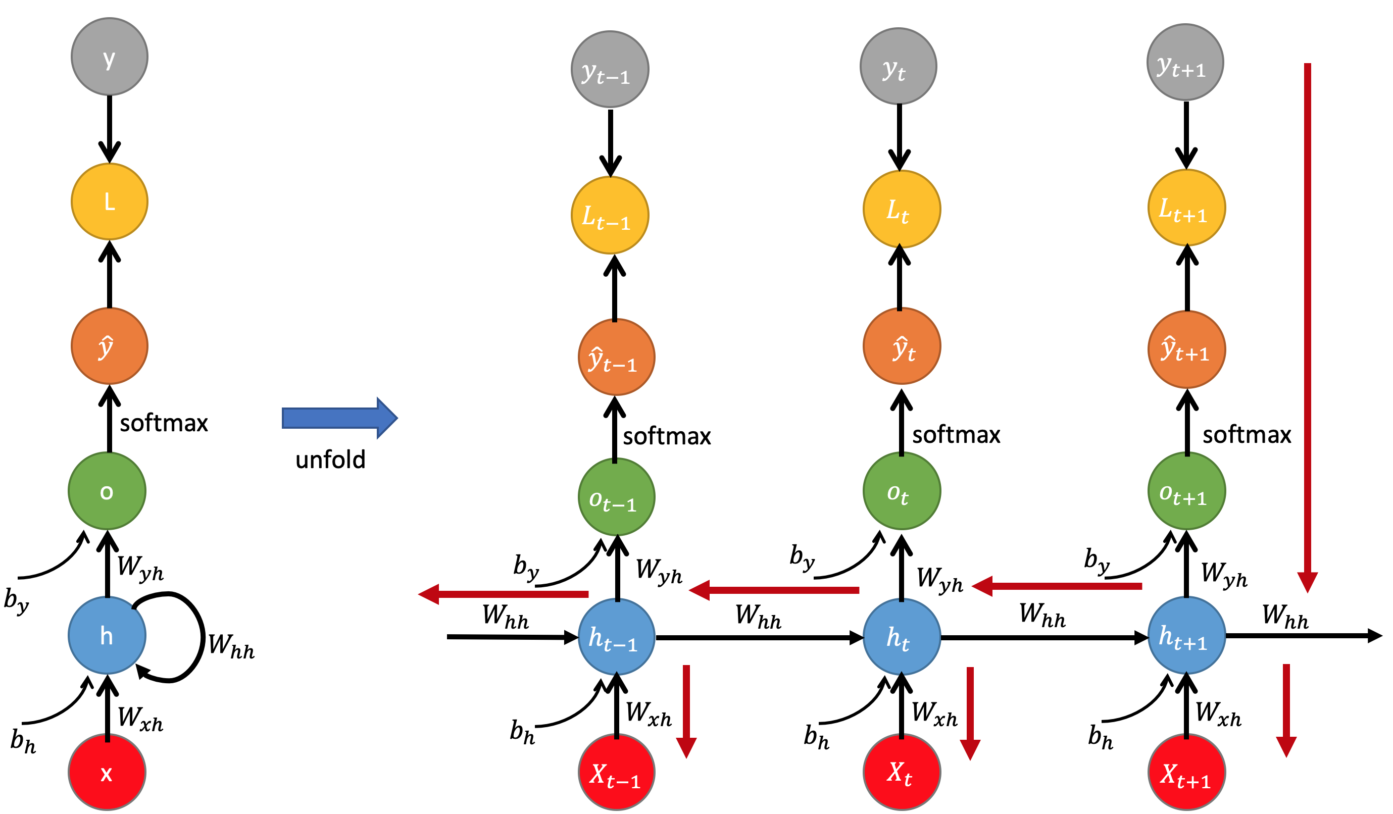
Suppose a model receives a sequence of input vectors $x_1,x_2,\dots ,x_T$. For a stream of measurements, $x_t$ might contain all features observed at step $t$. An RNN maintains a hidden state $h_t$: a fixed-size vector computed from the current input and the preceding state. It starts from an initial state $h_0$, often set to zero at the beginning of an independent sequence.

Watch how the same computation is reused at each step. The lecture uses words as inputs, but its architecture applies equally to numerical feature vectors.

To derive the update, we need a way to combine two sources of information: the new input $x_t$ and the previous state $h_{t-1}$. Give each source a learned linear transformation, add a bias, and apply a componentwise nonlinearity:

This is the vanilla RNN hidden-state recurrence. If $x_t\in {\mathbb{R}}^d$ and $h_t\in {\mathbb{R}}^m$, then $W_{xh}$ has shape $m\times d$, $W_{hh}$ has shape $m\times m$, and $b_h$ has length $m$. The tanh function acts on each entry of $a_t$. An optional output projection makes a prediction, for example,

The matrices are shared across time. There is one $W_{hh}$, not a newly learned matrix for every $t$. Consequently, the parameter count does not increase with sequence length, although processing a longer sequence takes more computation.

A two-step expansion makes the dependence on history explicit:

The first input can influence $h_2$, and therefore a prediction at step 2, only through the state carried forward. The same principle extends to later steps. It does not guarantee that useful information survives indefinitely: every update transforms the state again.

Why training has a long backward path

Consider a loss ${\ell }_T$ on a prediction made at the final step. A change to an early hidden state affects that loss through every intervening state. Backpropagation through time (BPTT) applies the ordinary chain rule to this unfolded computation.

The following reading makes an important distinction: a shared weight affects the state directly at the current step and indirectly through earlier states. You do not need to memorize its general product-and-sum notation; track those two routes of influence.

For our tanh recurrence, define the Jacobian of one state update with respect to the preceding state:

The expression $1-h_t^2$ is componentwise. It comes from the derivative of tanh: if a component of $h_t$ is near $1$ or $-1$, its corresponding derivative is near zero. Thus, even a sizeable recurrent weight need not transmit much gradient when the activation is saturated.

For an earlier step $k<T$, repeated use of the chain rule gives

Using column gradients, the part of the final loss signal reaching $h_k$ is

There are $T-k$ Jacobians in that product. Sequence length matters because the gradient must survive repeated multiplication, not because the model acquires more parameters.

The hidden states themselves are not the parameters we train, so why inspect their gradients? The signal reaching $h_k$ also determines how much the final loss can teach a weight used around step $k$. Because $W_{hh}$ is reused, its total gradient adds contributions from all its uses. A tiny distant contribution can be overshadowed by nearer ones even when the overall parameter gradient is not tiny.

Shrinking and growing products

In a one-dimensional RNN, a single backward step multiplies the gradient by

Imagine, just for illustration, that this factor stays near $0.72$. Across 50 steps, the distant signal is scaled by approximately $0.72^{50}$, or $7.5\times 10^{-8}$. This is a vanishing gradient: a late loss provides almost no guidance about how to change an early influence. If instead the factor stays near $1.35$, its product across 50 steps is about $3.3\times 10^6$. This is an exploding gradient, which can produce unstable parameter updates. Real Jacobians vary from step to step; the examples illustrate what persistent contraction or amplification does.

The matrix case has the same principle, with an important qualification. Since tanh derivatives have magnitude at most one,

Thus, if the spectral norm $\Vert W_{hh}{\Vert }_2$ is below one, the norm of a gradient travelling through many such steps is bounded by a geometrically shrinking quantity. A norm above one, however, does not guarantee explosion: the activation derivatives may be small, and successive matrices may amplify different directions. What matters is the product of the actual Jacobians along the sequence.

Watch the next excerpt for the visual chain-rule argument and its consequence for learning from distant observations. Its simplified weight-magnitude discussion is intuition, rather than a guarantee for every matrix and sequence.

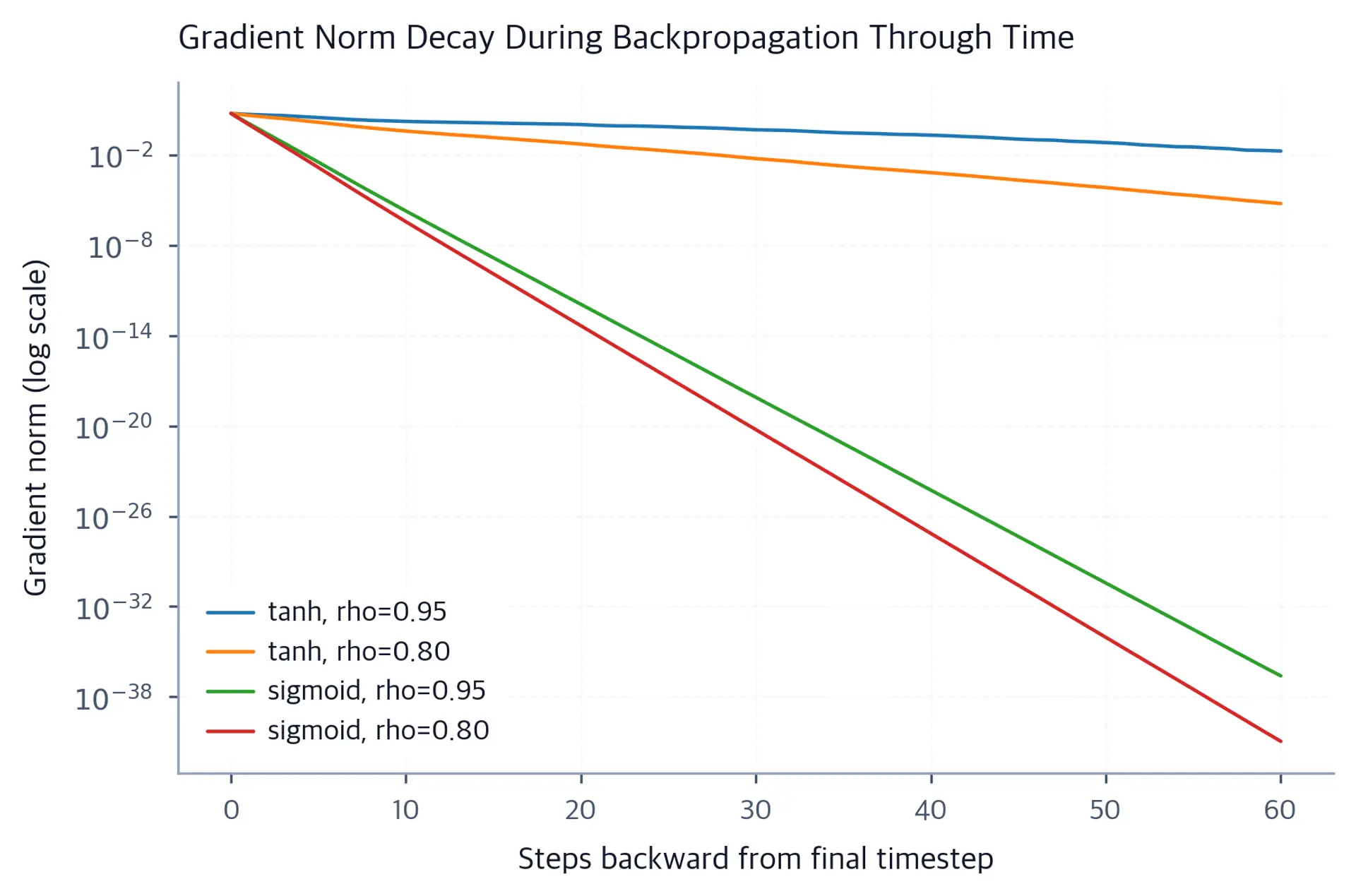
Sigmoid has a derivative no greater than $1/4$, while tanh can have a derivative near one around zero. That helps explain the contrast in the plotted settings, but tanh can also saturate and cause vanishing gradients. Likewise, a graph labeled by a weight matrix’s spectral radius cannot, by that label alone, predict every gradient: the activation values and the directions encountered during backpropagation matter too.

For a long measurement stream, the practical distinction is between processing an early observation and learning to use it later. The forward recurrence can accept the observation and continue updating its state. If the relevant backward signal vanishes, training struggles to adjust the model so that observation remains useful many steps later. If gradients explode, updates can instead become erratic or numerically invalid.

Takeaways

A vanilla RNN repeatedly applies one learned update to the current input and previous hidden state. Unfolding that update reveals why a late loss depends on early states through a product of many Jacobians. Persistent contraction makes long-range learning weak; persistent amplification can destabilize training. Neither outcome follows from sequence length alone—the weights, activations, and states jointly determine the gradient path.

Later in this sprint, you will use a gated recurrent model and control the length and magnitude of training gradients. First, the next lesson tackles a separate practical constraint: streaming sequence-sized groups from Parquet into PyTorch without loading the entire dataset into memory.