Knapsack DP: Subset Sum & Partition

Welcome to the next step in your journey through dynamic programming. In our last lesson, we focused on a crucial optimization, taking the 0/1 Knapsack solution from O(n * W) space down to an elegant O(W) by using a single 1D array and a backward-iterating loop. This wasn't just a memory-saving trick; it was about deeply understanding the data dependencies within a DP problem.

Today, we'll see that powerful pattern in action again, but in a completely new context. You'll learn to recognize how problems that don't mention "knapsacks," "weights," or "values" can often be solved using the very same 0/1 Knapsack logic. We will apply this pattern to solve two classic problems: the Subset Sum problem and the Partition Equal Subset Sum problem. Mastering this will significantly sharpen your ability to spot underlying DP patterns during coding interviews.

From Knapsacks to Subsets: The Core Connection

At its heart, the 0/1 Knapsack problem is about making a sequence of decisions. For each item, you have two choices: "take it" or "don't take it". The goal is to maximize value without exceeding a capacity constraint.

The Subset Sum problem asks something slightly different: given a set of numbers and a target sum, can you find a subset of those numbers that adds up exactly to the target?

Let's frame this as a 0/1 Knapsack problem:

• Items: The numbers in the input array.
• Weights of items: The value of each number itself.
• Values of items: Also the value of each number. Since we only care about the sum, weight and value are the same.
• Knapsack Capacity: The target sum.
• Goal: Instead of maximizing value, our goal is to determine if it's possible to pick a subset of items whose total weight is exactly equal to the capacity.

This reframing reveals that Subset Sum is a variation of the 0/1 Knapsack theme. We are still making a "take" or "don't take" decision for each number.

The "take U forward" channel has a great video that builds the logic for Subset Sum from the ground up using the "take/not take" recurrence.

The Dynamic Programming Formulation for Subset Sum

Let's formalize this with dynamic programming. We can define a boolean DP table, dp[i][j], which will be True if a sum of j can be achieved using a subset of the first i numbers, and False otherwise.

The recurrence relation is a direct translation of the "take/don't take" logic:
dp[i][j] = dp[i-1][j] (the "don't take" case: we can make sum j without the current number)
OR
dp[i-1][j - num[i-1]] (the "take" case: we can make the remaining sum j - num[i-1] with the previous numbers).

This leads to the full relation:

$$dp[i][j]=dp[i-1][j]\vee dp[i-1][j-{\text{num}}_{i-1}]$$

This is strikingly similar to the Knapsack recurrence, but we use a logical OR instead of max() because we are answering a boolean question ("Is it possible?") rather than an optimization one ("What is the maximum value?").

To see how this is built into a 2D table, the GeeksforGeeks article provides a clear walkthrough.

The Space-Optimized Solution

Just as with the 0/1 Knapsack problem, you might notice that to compute row i, we only ever need data from row i-1. This means we can apply the exact same space optimization! We can use a single 1D DP array, dp, of size target_sum + 1.

To preserve the 0/1 property (using each number at most once), we must again iterate the inner loop for the sums backwards. If we were to iterate forwards, we might use the same number multiple times within the same subproblem, which would incorrectly solve the Unbounded Subset Sum problem.

The NeetCode article on the related Partition Equal Subset Sum problem has an excellent, concise section explaining this optimal solution.

Here's a Python implementation for Subset Sum that uses this optimized approach.

def subset_sum(nums: list[int], target: int) -> bool:



    # dp[j] will be True if sum j is achievable
    dp = [False] * (target + 1)
    



    # Base case: a sum of 0 is always achievable with an empty set
    dp[0] = True
    
    for num in nums:



        # Iterate backwards to maintain the 0/1 property
        for j in range(target, num - 1, -1):



            # If we can make sum 'j' already, it stays True.
            # Otherwise, we check if we can make sum 'j' by including the current 'num'.
            # This is possible if we could previously make the sum 'j - num'.
            dp[j] = dp[j] or dp[j - num]
            
    return dp[target]




# Example
print(f"Can we make sum 9 from [3, 34, 4, 12, 5, 2]? {subset_sum([3, 34, 4, 12, 5, 2], 9)}") # True
print(f"Can we make sum 30 from [3, 34, 4, 12, 5, 2]? {subset_sum([3, 34, 4, 12, 5, 2], 30)}") # False

Application: Partition Equal Subset Sum

Now let's tackle the next problem: Can a given array of positive integers be partitioned into two subsets with an equal sum?

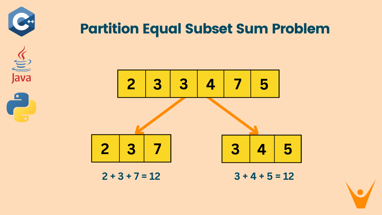
This might seem different, but a key insight reduces it directly to the Subset Sum problem.

1. Let the total sum of all numbers in the array be S.
2. If we partition the array into two subsets, S1 and S2, with equal sums, then sum(S1) = sum(S2).
3. Since S1 and S2 together contain all original elements, sum(S1) + sum(S2) = S.
4. This means 2 * sum(S1) = S, or sum(S1) = S / 2.

This leads to two crucial observations:

• An equal partition is impossible if the total sum S is odd. We can immediately return False.
• If S is even, the problem is equivalent to asking: "Is there a subset in the original array that sums up to S / 2?"

This is precisely the Subset Sum problem we just solved!

The following video explains this reduction very clearly.

The algorithm is therefore straightforward:

1. Calculate the total sum of the array.
2. If the sum is odd, return False.
3. Define the target as total_sum / 2.
4. Use the subset_sum logic to determine if a subset with this target sum exists in the array.

Here is the complete implementation in Python:

def can_partition(nums: list[int]) -> bool:
    total_sum = sum(nums)
    



    # 1. If the total sum is odd, we can't partition it into two equal halves.
    if total_sum % 2 != 0:
        return False
        



    # 2. The target for our subset sum is half of the total sum.
    target = total_sum // 2
    



    # 3. Now, this is just the Subset Sum problem.
    dp = [False] * (target + 1)
    dp[0] = True
    
    for num in nums:
        for j in range(target, num - 1, -1):
            dp[j] = dp[j] or dp[j - num]
            
    return dp[target]




# Example from the image
print(f"Can [2, 3, 3, 4, 7, 5] be partitioned equally? {can_partition([2, 3, 3, 4, 7, 5])}") # True
print(f"Can [1, 5, 11, 5] be partitioned equally? {can_partition([1, 5, 11, 5])}") # True (11 vs 1+5+5)
print(f"Can [1, 2, 3, 5] be partitioned equally? {can_partition([1, 2, 3, 5])}") # False

Note how the core DP logic inside can_partition is identical to the subset_sum function.

Finding the Subset (An Aside)

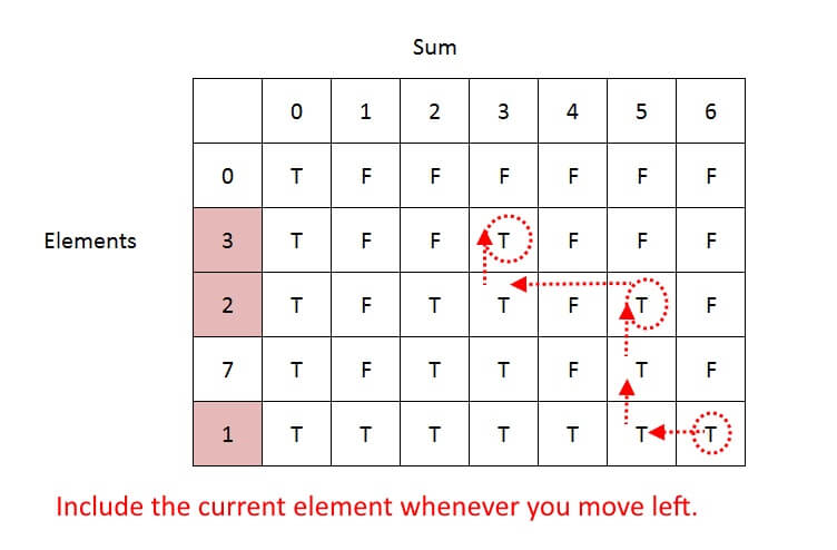
Our DP solution efficiently answers if a partition is possible, which is what these LeetCode-style problems usually ask. If you needed to find the actual numbers in the subset, you would need to backtrack through the 2D DP table (the 1D optimization loses this path information). You would start from dp[n][target] and trace your steps backward to see which decisions (take or not take) led to the True result.

Conclusion

In this lesson, we saw how the fundamental 0/1 Knapsack pattern extends beyond its initial framing. By recognizing the core "take/don't take" decision structure, we could solve two new problems, Subset Sum and Partition Equal Subset Sum.

Key Takeaways:

• Problem Reduction: The Partition Equal Subset Sum problem elegantly reduces to the Subset Sum problem if the total sum is even.
• Pattern Recognition: Subset Sum is a variation of the 0/1 Knapsack problem where weights and values are the same, and the goal is to check for feasibility (True/False) rather than maximizing a value.
• The 1D DP Template: The space-optimized 1D DP solution with a backward inner loop is a robust template for all 0/1-style decision problems. The direction of this loop is critical and distinguishes it from another major DP pattern.

In our last lesson, we noted that iterating the inner loop forward would break the 0/1 property. In our next lesson, we will explore exactly that: the Unbounded Knapsack problem, where you can take items multiple times. We will see how a simple change in the loop's direction—from backward to forward—unlocks the solution to a whole new class of problems.