Recommended resources
The freely available resources this lesson will direct you to.
Welcome back! In our last lesson, we established a blueprint for converting recursive, memoized DP solutions into iterative, bottom-up ones. You learned that both approaches solve the same subproblems, but tabulation does so by systematically building up from the base cases, often leading to better performance.
Today, we'll apply this knowledge to one of the most famous problems in computer science: the 0/1 Knapsack problem. This problem serves as a gateway to 2D dynamic programming and is a powerful pattern for solving a wide range of resource allocation puzzles. Given your interest in finance, you can think of it as a simplified model of portfolio construction: you have a limited budget (the knapsack's capacity) and a set of potential investments (items), each with a cost (weight) and an expected return (value). Your goal is to choose the combination of investments that maximizes your total return without exceeding your budget.
Our objective is to formulate the recurrence relation for the 0/1 knapsack problem and then implement a solution using a 2D DP table, solidifying the bottom-up approach we studied previously.
Understanding the 0/1 Knapsack Problem
The problem is defined as follows: you are given a set of items, each with a specific weight and value. You also have a knapsack that can hold a certain maximum weight. Your task is to select a subset of these items to put into the knapsack such that the total value of the selected items is maximized, and their total weight does not exceed the knapsack's capacity. The "0/1" constraint means that for each item, you have two choices: either you take the whole item (1) or you leave it behind (0). You cannot take a fraction of an item.
The following resource provides a clear and structured introduction to the problem.
This article from Hello Algo formally defines the 0/1 Knapsack problem and frames it as a series of decisions, which is a perfect setup for a dynamic programming approach.
Read the introductory section, up to but not including "Step 1". Focus on understanding the inputs (the problem statement) and why it fits a decision-making model.
Like the problems we've seen before, the 0/1 Knapsack problem exhibits the two key properties that make it suitable for dynamic programming:
- Optimal Substructure: The optimal solution to the problem (for
nitems and capacityW) contains within it the optimal solutions to smaller subproblems (e.g., forn-1items). - Overlapping Subproblems: A naive recursive approach would repeatedly solve the same subproblems. For example, the maximum value for the first 3 items with a remaining capacity of 10 might be needed in many different decision paths.

Formulating the Recurrence Relation
To solve this with DP, we first need to define the state and the recurrence relation. This is the most crucial part of solving any DP problem. We'll follow the structured thinking from our last lesson.
1. Define the State
At any point, what information do we need to make a decision? We need to know which item we are currently considering and how much capacity we have left in the knapsack. This leads to a two-dimensional state: (i, c), representing the subproblem of finding the maximum value using only the first i items with a knapsack of capacity c.
Let's define dp[i][c] as the solution to this subproblem. Our goal is to find dp[n][W], where n is the total number of items and W is the total capacity of the knapsack.
2. Define the Choices
For each item i, we face a decision with two possible outcomes:
-
Choice A: Do not include item
iin the knapsack.
If we don't take itemi, then the maximum value we can get is simply the best we could do with the previousi-1items, using the same capacityc. The value for this choice isdp[i-1][c]. -
Choice B: Include item
iin the knapsack.
We can only make this choice if the weight of itemi(wgt[i-1]) is less than or equal to the current capacityc. If we take it, we gain its value (val[i-1]), but we use upwgt[i-1]of our capacity. The remaining value must come from the optimal solution for the firsti-1items with the reduced capacityc - wgt[i-1]. The value for this choice isval[i-1] + dp[i-1][c - wgt[i-1]].
3. The Recurrence Relation
Since we want to maximize the value, we simply take the maximum of these two choices. This gives us our state transition equation.
The resource from Hello Algo walks through this derivation beautifully.
This reading formally defines the DP state and derives the state transition equation based on the two choices for each item.
Read through Step 1 and Step 2 in the article. Pay close attention to how the state dp[i, c] is defined as the solution to a subproblem and how this leads directly to the state transition equation by considering the two cases (put the item in or not).
So, the full recurrence relation is:
- If
wgt[i-1] > c(itemiis too heavy):
- If
wgt[i-1] <= c:
Bottom-Up Implementation with a 2D Table
Now, let's build the solution iteratively using a 2D DP table. This process will feel very familiar from our last lesson, but now applied to a 2D state.
-
Create the DP Table: Our state
(i, c)has two parameters. We'll use a 2D array, let's call itdp, of size(n+1) x (W+1), wherenis the number of items andWis the knapsack capacity.dp[i][j]will store the max value using the firstiitems with capacityj. -
Initialize Base Cases: The "Hello Algo" resource mentions this in Step 3. When there are no items (
i=0) or the capacity is zero (c=0), the maximum value is 0. This means the entire first row (dp[0][c]) and the entire first column (dp[i][0]) of our table should be initialized to 0. Most programming languages will default-initialize a new integer array to zeros, so this is often handled for us. -
Iterate and Apply Recurrence: Our recurrence
dp[i][c]depends on values in the previous row (i-1). This tells us our outer loop must iterate over the items, and the inner loop over the capacities.- Outer loop for
ifrom1ton. - Inner loop for
cfrom1toW. - Inside the loops, we implement the
if/elselogic of our recurrence relation.
- Outer loop for
The following video provides an exceptionally clear, step-by-step walkthrough of filling this 2D table. It masterfully explains the meaning of each cell as the answer to a specific subproblem, which is key to demystifying the process.
The 0/1 Knapsack Problem (Demystifying Dynamic Programming)
This Back To Back SWE video is one of the best explanations of the 0/1 Knapsack problem. It focuses on the logic behind each step rather than just mechanical formula application.
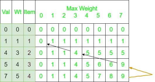
First, watch the explanation of the DP table structure and the recurrence relation from the initial setup. The presenter clearly defines the two choices at each step. Next, follow along with the detailed, cell-by-cell walkthrough of filling the table from the table-filling process. Pay close attention to how each cell's value is determined by comparing the two choices: Don't take the current item: The value is inherited from the cell directly above (dp[i-1][c]). Take the current item: The value is the current item's value plus the value from the cell in the previous row, shifted left by the current item's weight (val[i-1] + dp[i-1][c - wgt[i-1]]). The final value in the bottom-right corner of the table, dp[n][W], is the answer to our original problem.
Here is a clean Python implementation that matches the logic we've just discussed. The final answer is the value in the bottom-right corner of the dp table.
This section provides the complete bottom-up DP code.
Review the Python implementation. See how it directly translates our 3-step process: dp = [[0] * (cap + 1) for _ in range(n + 1)]: Creates and initializes the (n+1) x (cap+1) table. The nested loops (for i in range(1, n + 1) and for c in range(1, cap + 1)) implement the bottom-up build order. The if/else block inside the loops is the direct implementation of our recurrence relation.
The image below shows an example of a filled DP table. The arrows illustrate how the value in a cell is derived from values in the previous row, corresponding to the "don't take" and "take" decisions.
Complexity Analysis
- Time Complexity: We are filling a 2D table of size
(n+1) x (W+1). Since we perform a constant amount of work for each cell, the total time complexity isO(n * W). - Space Complexity: We need to store the entire 2D table, so the space complexity is also
O(n * W).
An interesting point for a CS major: this complexity is called pseudo-polynomial. The runtime depends not just on the number of items n, but on the magnitude of the capacity W. If W is extremely large (e.g., 2^n), the algorithm's runtime can become exponential relative to the size of the input representation.
Conclusion
In this lesson, we tackled the classic 0/1 Knapsack problem. By applying the DP principles from our previous sessions, you learned how to handle a problem with a two-dimensional state, a common pattern in more advanced DP challenges.
Key Takeaways:
- Problem Definition: The 0/1 Knapsack problem asks for the maximum value of items that can fit into a weight-constrained bag, where items are indivisible.
- State Formulation: The problem requires a 2D state,
dp[i][c], representing the maximum value achievable with the firstiitems and a capacity ofc. - Recurrence Relation: The core logic lies in the choice for each item: either we don't take it (
dp[i-1][c]) or we take it (val[i-1] + dp[i-1][c - wgt[i-1]]). The DP state is the maximum of these two options. - 2D Table Implementation: A bottom-up solution involves iterating through items and capacities to fill an
(n+1) x (W+1)table, with the final answer located atdp[n][W].
The O(n * W) space complexity of our solution is correct, but for interviews, it's often expected that you can do better. In our next lesson, we will explore a common and clever optimization that reduces the space complexity of the 0/1 Knapsack solution to just O(W), a significant improvement. This technique relies on a careful analysis of the data dependencies within the DP table.