Estimating AI Workload Infrastructure Demands

Hello! In the previous lesson, you traced data, artifacts, and control decisions through an AI system. That trace is now a capacity-planning tool: once you know what runs, where it runs, and what it moves, you can estimate the infrastructure it needs.

This lesson builds a first-pass estimate for a representative training job across four dimensions: compute, accelerator memory, network, and storage. We’ll then contrast it briefly with inference, where the same model can create a very different resource profile. The goal is not a precise hardware purchase recommendation; it is an estimate whose assumptions are visible and testable.

---

Start with a workload contract, not an accelerator specification

Suppose you need to fine-tune a roughly one-billion-parameter transformer on one billion tokens, using four accelerators. This is an illustrative workload, not a prescription for the recommendation system from the previous lesson. We will assume:

• Each accelerator has 32 GB of device memory and a theoretical 200 trillion BF16 floating-point operations per second for the operations this model uses.
• Training uses an Adam-style optimizer and ordinary replicated data parallelism: every accelerator holds a model copy and processes different examples.
• Each accelerator processes two sequences of 2,048 tokens per step. There is no gradient accumulation.
• A single accelerator sustains 30% of the relevant theoretical compute peak on this workload. Adding four accelerators retains 80% scaling efficiency relative to that single-accelerator rate.
• Training input is already packed as four-byte token IDs. These rates and efficiencies are planning assumptions; benchmarks must replace them before a capacity commitment.

The global batch is $4\times 2\times 2,048=16,384$ tokens per step, so the run takes approximately 61,036 steps. Keeping that batch definition explicit matters: changing sequence length or the number of sequences per accelerator changes activation memory and step count, even if the model has not changed.

A useful capacity estimate has two parts. Demand describes work or bytes the job requires. Supply describes the rate and capacity actually available at each boundary. Compare like units—FLOPs with FLOP/s, bytes with GB of memory, and bytes per step with bytes/s of network or storage throughput. A job can satisfy its total storage-capacity requirement yet still stall on checkpoint write speed.

---

Compute: estimate useful work, then elapsed time

For a dense transformer, a common first approximation for training is six FLOPs per parameter per training token. It covers the dominant forward and backward matrix operations. It is less reliable for unusual architectures or very long sequences where attention work becomes relatively important.

For our workload:

$$F_{\text{train}}\approx 6PD=6(10^9)(10^9)=6\times 10^{18}\text{FLOPs},$$

where $P$ is parameter count and $D$ is the number of tokens processed across the run. This is useful model work, not a claim that the hardware performs only those operations. Data preparation, communication, and any activation recomputation add work or time.

The assumed effective useful compute rate is:

$$R_{\text{useful}}=4(200\times 10^{12})(0.30)(0.80)=192\times 10^{12}\text{FLOP/s}.$$

The resulting first-pass runtime is:

$$T_{\text{train}}\approx \frac{6\times 10^{18}}{192\times 10^{12}}=31,250\text{s}\approx 8.7\text{hours}.$$

That implies about 0.51 seconds per step. Treat it as a target to interrogate, not a guaranteed completion time. The 30% assumption represents sustained single-accelerator model throughput, while the 80% factor represents the additional loss from distributing this job. If you measure end-to-end model FLOPs utilization on the four-accelerator job, it already incorporates many of those losses; multiplying by another scaling factor would double-count them.

This distinction is useful operationally. If a trial run takes 0.8 seconds per step rather than 0.51, adding accelerators is not the first diagnosis. Compare measured accelerator work, input wait, synchronization wait, and checkpoint pauses to find which assumption failed.

---

Accelerator memory: separate persistent state from the batch-dependent peak

Compute time answers how long? Device memory first answers will it run at all? Replicated data parallelism means that each of our four accelerators needs its own copy of the training state. Four 32 GB devices do not give one replica a contiguous 128 GB memory pool.

Assume BF16 weights and gradients, plus an FP32 master-weight copy and two FP32 optimizer moments. Per parameter, that is:

State held on each accelerator	Bytes per parameter
BF16 weights and BF16 gradients	$2+2$
FP32 master weights	$4$
Two FP32 optimizer moments	$4+4$
Total during training	16

For one billion parameters, persistent training state is therefore about 16 GB per accelerator. This is an assumption about the optimizer implementation, not a universal constant: gradient precision, optimizer layout, and temporary copies can change it.

Next come activations, intermediate values retained so the backward pass can compute gradients. An initial sizing term is the size of one hidden-state tensor at one layer:

$$M_{\text{hidden}}=B_{\text{local}}SHb=2(2,048)(2,048)(2)\approx 16.8\text{MB},$$

where $B_{\text{local}}$ is sequences per accelerator, $S$ is sequence length, $H$ is hidden width, and $b$ is bytes per element. This is not the full activation footprint. Attention, feed-forward operations, and framework choices retain additional tensors.

For planning, suppose this model has 16 layers and the retained activations average eight such tensors per layer. That gives approximately 2.15 GB. The factor of eight is an explicit placeholder to replace with a measured peak; in particular, attention implementation can materially change memory use. Allow another 2 GB for runtime and temporary buffers, then add 25% headroom:

$$M_{\text{planned}}\approx (16+2.15+2)\times 1.25\approx 25.2\text{GB per accelerator}.$$

On the assumed 32 GB device, this appears feasible, with limited room for an unexpectedly larger activation peak. Increasing local batch size primarily raises activation demand; increasing parameter count raises weights, gradients, and optimizer-state demand. Longer sequences also increase activations, sometimes more sharply than this simple linear term suggests.

The image below shows one way to respond if activations become the binding constraint. Activation checkpointing saves selected intermediate values and recomputes others during backpropagation. Its “checkpoints” live in the computation’s memory-management strategy; they are not the durable files used to restart a failed training job.

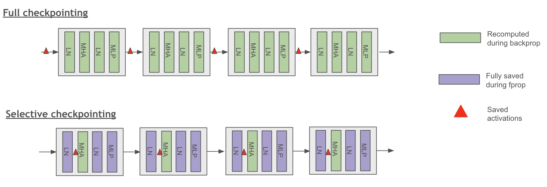
This trade can make an otherwise impossible batch fit, but recomputation can increase elapsed time. If you enable it, revise the runtime estimate rather than treating memory savings as free.

The following reading gives context for the memory rule of thumb, distributed communication, and a crucial distinction between in-memory training state and on-disk recovery state. Its hardware examples are reference points, not specifications for our hypothetical devices.

---

Network: count traffic at each synchronization boundary

The previous lesson’s flow trace tells us which data crosses a boundary. For this replicated data-parallel job, every accelerator computes gradients on different examples; the replicas must combine those gradients before updating their matching weights. That synchronization is the dominant recurring accelerator-to-accelerator traffic in this simple design.

Watch this short portion of the lecture to connect the algorithm to the infrastructure demand. The full lecture covers more elaborate parallelism strategies; we need only the replicated-model case here.

If gradients occupy two bytes per parameter, the gradient message is about 2 GB. For a four-participant ring AllReduce, the bandwidth-oriented estimate from the reading is:

$$M_{\text{ring, per participant}}\approx \frac{2(N-1)}{N}M=\frac{2(4-1)}{4}(2\text{GB})=3\text{GB}.$$

This is approximately 3 GB sent per accelerator per step, with a comparable amount received. It is not 3 GB for the entire cluster, and it is not necessarily a single transfer. Gradient precision or a different synchronization algorithm changes the number.

At the target 0.51 seconds per step, each accelerator would average about 5.9 GB/s of outgoing collective traffic, plus comparable incoming traffic. Suppose its usable interconnect delivers 25 GB/s per direction during the collective. The idealized bandwidth-only floor for sending 3 GB is about 0.12 seconds, before collective latency, contention, or topology effects.

That 0.12-second floor is significant beside a 0.51-second step. Our 80% scaling-efficiency assumption is plausible only if communication can be substantially overlapped with backward computation, or if the measured collective performs better than this conservative comparison suggests. Network bytes alone cannot prove the step-time estimate. A brief benchmark should record collective duration, overlap, effective bandwidth, and the slowest participant—not just average NIC utilization. Peak bursts can be important even when the step-averaged rate looks modest.

Network demand also depends on placement. If all participants communicate over a fast local interconnect, one capacity estimate applies; if synchronization crosses nodes and a slower fabric, use that fabric’s effective rate. More elaborate sharding or model parallelism changes both memory occupancy and what must cross these links. Those choices come later in the course; the sizing habit remains the same: identify each recurring transfer, its bytes, its frequency, and its actual network tier.

---

Storage: distinguish retained bytes from bytes per second

The tokenized training snapshot is small relative to model state: one billion token IDs at four bytes each occupy about 4 GB before metadata, indexes, or compression. Spread over 8.7 hours, the average input payload rate is only about 128 KB/s for the whole job. That does not prove the input pipeline is healthy. Many tiny objects, expensive decoding, insufficient prefetching, or uneven sharding can stall accelerators despite a low average byte rate.

Recovery storage is a different calculation. A checkpoint containing BF16 weights, FP32 master weights, and two FP32 optimizer moments is approximately 14 bytes per parameter, or 14 GB for this model. Gradients are needed during an active step but ordinarily need not be retained in this recovery artifact. Saving one complete checkpoint from each of four identical replicas would unnecessarily multiply storage; this estimate assumes one logical checkpoint per save.

If you retain three checkpoints, that is approximately 42 GB. Allowing two 4 GB data copies—for example, a prepared snapshot and a separately retained staging copy—and a 2 GB exported BF16 model gives an illustrative retained footprint of about 52 GB, before logs, filesystem overhead, replication, and backups. Artifact-retention policy therefore matters more here than raw token volume.

Capacity and write rate must be assessed separately. At a genuinely available aggregate write rate of 1 GB/s, a 14 GB checkpoint has a 14-second bandwidth-only minimum. One save per hour would spend at least about 0.4% of wall time writing if saves block training throughout. Real pause time can be higher because checkpoint creation and serialization have costs; asynchronous writes may hide some of it but can require extra memory or staging space. Checkpoint frequency, recovery objectives, and retention will receive their own treatment later. For now, make both GB retained and seconds per save visible in the estimate.

---

A compact, reproducible estimate—and why inference differs

You can keep the assumptions in a small script rather than burying them in a cluster request. This version uses decimal GB and intentionally exposes its uncertain activation and efficiency factors:

import math

parameters = 1e9
tokens = 1e9
accelerators = 4
peak_flops_per_s = 200e12
single_accelerator_mfu = 0.30
scaling_efficiency = 0.80

sequences_per_accelerator = 2
sequence_length = 2048
hidden_width = 2048
layers = 16
saved_tensor_factor = 8

global_tokens_per_step = (
    accelerators * sequences_per_accelerator * sequence_length
)
steps = math.ceil(tokens / global_tokens_per_step)
training_flops = 6 * parameters * tokens
run_seconds = training_flops / (
    accelerators * peak_flops_per_s
    * single_accelerator_mfu * scaling_efficiency
)

state_bytes = parameters * (2 + 2 + 4 + 4 + 4)
activation_bytes = (
    layers * saved_tensor_factor * sequences_per_accelerator
    * sequence_length * hidden_width * 2
)
planned_device_bytes = (state_bytes + activation_bytes + 2e9) * 1.25

gradient_bytes = parameters * 2
ring_bytes_sent_per_step = (
    2 * (accelerators - 1) / accelerators * gradient_bytes
)
checkpoint_bytes = parameters * (2 + 4 + 4 + 4)

print(f"Steps: {steps:,}; run: {run_seconds / 3600:.1f} hours")
print(f"Planned memory/device: {planned_device_bytes / 1e9:.1f} GB")
print(f"Ring bytes sent/device/step: {ring_bytes_sent_per_step / 1e9:.1f} GB")
print(f"One checkpoint: {checkpoint_bytes / 1e9:.1f} GB")

The expected order of magnitude is 61,036 steps, 8.7 hours, 25.2 GB per accelerator, 3 GB sent per accelerator per step, and 14 GB per checkpoint. An implementation-oriented next step is to replace the assumed factors with observations from a short run: peak allocated device memory, tokens/s, step time, collective timing, input wait, and checkpoint duration. Keep the workload definition fixed while comparing estimate with measurement; otherwise, a faster result might simply reflect less work.

It is worth checking the opposite workload shape before generalizing these training numbers to serving. In autoregressive LLM inference, weights stay resident, but each concurrent request also needs a growing key-value (KV) cache. The following video illustrates how memory movement and cache occupancy can limit generation even when substantial arithmetic capacity is available.

For instance, seven billion BF16 weights alone occupy about 14 GB. Unlike training, inference does not normally keep gradients and Adam moments resident; unlike the simple training-state calculation, its active-request memory grows with concurrency and context length. That is why “fits the model weights” does not mean “serves the target traffic.” Later lessons will estimate that cache and the serving latency-throughput trade-off in detail.

---

Conclusion

A defensible first-pass workload estimate keeps four accounts separate:

• Compute: total useful work, sustained—not peak—rate, and implied runtime.
• Accelerator memory: per-device training state, batch-dependent activations, runtime buffers, and headroom.
• Network: bytes per synchronization, frequency, placement, and whether transfers fit within step time.
• Storage: retained datasets and artifacts as well as input and checkpoint transfer rates.

The estimates here are useful precisely because their uncertain assumptions are named. A short benchmark can turn them into measured capacity requirements instead of an unexplained accelerator count. Next, you’ll separate the control plane that admits and coordinates AI workloads from the data plane that moves data and performs the work; the resource boundaries you have quantified will make that architectural distinction more concrete.