Applying Bayes’ Theorem to Conditional Probability and Base Rates

Recommended resources

The freely available resources this lesson will direct you to.

Welcome to the first lesson in the mathematical-reasoning module. Over this module, you will refresh the probability, statistics, linear algebra, and optimization ideas that commonly appear in ML and MLOps interviews. The emphasis is not on memorizing formulas: it is on translating an ambiguous prompt into the right quantities, calculating cleanly, and explaining what the result means for a deployed ML system.

This lesson focuses on conditional probability, Bayes’ theorem, and the base-rate effect. These are especially relevant whenever an interviewer gives you a detector’s true-positive and false-positive rates and asks what an alert actually means in production.

Conditional probability: restrict the population first

Conditional probability answers a simple question:

Once we know that $B$ happened, what fraction of the remaining cases also satisfy $A$ ?

It is written:

P (A ∣ B)

and read as “the probability of $A$ , given $B$ .”

The formal definition is:

P (A ∣ B) = \frac{P ( A \cap B )}{P ( B )}

provided that $P (B) > 0$ .

The denominator is crucial. Conditioning on $B$ changes the reference population from all cases to only the cases where $B$ is true.

For example, suppose an object-detection service processes camera frames, and:

$A$ : a frame contains a pedestrian.
$B$ : the frame is captured at night.

Then $P (A ∣ B)$ is the probability that a frame contains a pedestrian among nighttime frames, not among all frames. If nighttime traffic patterns differ from daytime patterns, it can differ substantially from $P (A)$ .

Two expressions that look similar may represent very different questions:

Expression	Meaning
$P (A ∣ B)$	Probability of $A$ among cases where $B$ is known
$P (B ∣ A)$	Probability of $B$ among cases where $A$ is known

For a classifier:

P (alert ∣ hazard)

is its sensitivity or true-positive rate. But an operator usually cares about:

P (hazard ∣ alert)

the probability that an alert corresponds to a real hazard. These are not interchangeable.

The multiplication rule follows directly from the definition:

P (A \cap B) = P (A ∣ B) P (B)

This rule is the workhorse for Bayes problems. It says that a joint event has two components:

How common the starting condition is.
How likely the next observation is under that condition.

[PDF] Conditional Probability, Independence and Bayes' Theorem

Read MIT OpenCourseWare’s treatment of conditional probability, total probability, and the base-rate fallacy. It provides the formal vocabulary and the tree/table methods that are useful under interview time pressure.

In Section 2, begin with conditional probability. Focus on why the denominator becomes the restricted population and how the multiplication rule follows from the definition. Then read Section 4, beginning with the law of total probability. Notice that the total probability of an outcome is the sum of its mutually exclusive paths. In Section 7, read the derivation of Bayes’ rule. Finally, in Section 7.1, start at the base-rate warning and continue through the screening-test example, including its table-based solution. Compare the direction of every conditional probability before looking at the arithmetic.

Bayes’ theorem: update a prior using evidence

Bayes’ theorem reverses the direction of a conditional probability. Let:

$H$ be a hypothesis, such as “a real hazard is present.”
$E$ be observed evidence, such as “the perception system issued an alert.”

Bayes’ theorem is:

P (H ∣ E) = \frac{P ( E ∣ H ) P ( H )}{P ( E )}

For a binary hypothesis, where either $H$ or $H^{c}$ must be true, the denominator expands using the law of total probability:

P (H ∣ E) = \frac{P ( E ∣ H ) P ( H )}{P ( E ∣ H ) P ( H ) + P ( E ∣ H ^{c} ) P ( H ^{c} )}

Each term has a practical interpretation:

Quantity	Interpretation
$P (H)$	Prior: base rate before seeing evidence
$P (E ∣ H)$	Likelihood: how often the evidence appears if the hypothesis is true
$P (E)$	Overall frequency of the evidence
$P (H ∣ E)$	Posterior: updated probability after observing evidence

The numerator,

P (E ∣ H) P (H)

is the probability of both a real hazard and an alert. The denominator is the probability of any alert, whether it is a true positive or a false positive. The posterior is therefore the fraction of all alerts that are genuine.

A compact way to state the logic is:

Posterior probability is proportional to prior probability times how compatible the evidence is with the hypothesis.

The word proportional matters because all competing explanations for the evidence must be accounted for in the denominator.

Bayes theorem, the geometry of changing beliefs

Watch 3Blue1Brown’s “Bayes theorem, the geometry of changing beliefs” for a visual, natural-frequency explanation of why evidence must update a base rate rather than replace it.

Watch natural frequencies to see how a representative population turns abstract probabilities into counts. Then watch formal Bayes, which maps the intuitive counts to hypothesis, evidence, prior, likelihood, and posterior. Pay particular attention to why the denominator includes every way the evidence could occur.

The base-rate effect in an ML alerting system

Consider an automotive-perception scenario. A forward-collision detector produces an alert for a genuinely hazardous object ahead.

Suppose that, for the operational unit you have defined:

A real hazard is present in $1%$ of evaluated driving windows:

P (H) = 0.01

The detector raises an alert in $95%$ of windows containing a real hazard:

P (E ∣ H) = 0.95

The detector still raises an alert in $4%$ of windows without a real hazard:

P (E ∣ H^{c}) = 0.04

An interviewer asks: Given an alert, what is the probability that a real hazard exists?

Apply Bayes’ theorem:

P (H ∣ E) = \frac{0.95 \times 0.01}{( 0.95 \times 0.01 ) + ( 0.04 \times 0.99 )}

P (H ∣ E) = \frac{0.0095}{0.0491} \approx 0.193

So only about $19.3%$ of alerts correspond to a genuine hazard.

That result may initially seem surprising because a $95%$ true-positive rate sounds strong. The reason is that non-hazard windows outnumber hazard windows by $99$ to $1$ . Even a modest false-positive rate can generate many false alerts.

Natural frequencies make this immediately clear. Imagine $10, 000$ representative driving windows.

Actual condition	Number of windows	Alert rate	Alerts
Real hazard	100	$95%$	95 true positives
No real hazard	9,900	$4%$	396 false positives
Total	10,000	—	491 alerts

Among the $491$ alerts, only $95$ are genuine:

P (H ∣ E) = \frac{95}{491} \approx 19.3%

A population-count decision tree: 180 true positives and 980 false positives result from a low-prevalence condition, illustrating why a positive result need not imply a high probability that the condition is present.

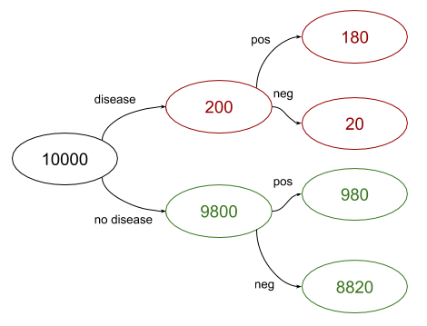
This is the base-rate effect. A low base rate does not mean the model is poor. It means that the meaning of a positive prediction depends jointly on:

how often the target event occurs in deployment;
the model’s true-positive rate;
the model’s false-positive rate;
the operational unit used to define prevalence, such as frames, scenes, trips, or safety-critical situations.

For perception systems, defining that unit carelessly can make a reported posterior misleading. Treating sequential video frames as independent, for example, can inflate the apparent sample size and obscure persistent false-positive bursts.

A reliable interview method

For most Bayes questions, use the same disciplined sequence.

1. Define events before calculating

State what the events mean.

For the perception example:

H = real hazard present

E = detector issues an alert

Then name the requested quantity:

P (H ∣ E)

This alone prevents the common mistake of returning $P (E ∣ H)$ , the sensitivity, because it was given in the prompt.

2. Identify the prior and likelihoods

Extract:

P (H), P (E ∣ H), P (E ∣ H^{c})

If the prompt states specificity rather than false-positive rate, convert it:

P (E ∣ H^{c}) = 1 - P (no alert ∣ H^{c})

3. Calculate each path’s probability

Compute the two joint masses:

P (E \cap H) = P (E ∣ H) P (H)

P (E \cap H^{c}) = P (E ∣ H^{c}) P (H^{c})

These represent true-positive and false-positive alert mass, respectively.

4. Normalize within the observed evidence

Add all paths that produce the observed evidence:

P (E) = P (E \cap H) + P (E \cap H^{c})

Then divide the target path by that total:

P (H ∣ E) = \frac{P ( E \cap H )}{P ( E )}

5. Interpret the answer operationally

Do not stop at the decimal. For example:

“Although recall is $95%$ , the alert precision in this deployment setting is only about $19%$ , because hazards occur in only $1%$ of windows. Before using this alert for an automatic braking action, I would examine false-positive costs and slice the calculation by speed, weather, road class, and sensor health.”

That is a stronger interview answer than formula substitution alone.

From classifier metrics to Bayesian quantities

Bayes’ theorem exposes a distinction that matters in production ML.

A confusion-matrix evaluation commonly estimates:

True-positive rate / recall / sensitivity

P (\hat{Y} = 1 ∣ Y = 1)

False-positive rate

P (\hat{Y} = 1 ∣ Y = 0)

But a product team often asks for precision or positive predictive value:

P (Y = 1 ∣ \hat{Y} = 1)

Precision is a Bayesian posterior. It depends on class prevalence:

P (Y = 1 ∣ \hat{Y} = 1) = \frac{P ( Y ^ = 1 ∣ Y = 1 ) P ( Y = 1 )}{P ( Y ^ = 1 ∣ Y = 1 ) P ( Y = 1 ) + P ( Y ^ = 1 ∣ Y = 0 ) P ( Y = 0 )}

This has an important deployment implication:

Precision measured on a balanced validation set may not transfer to a production population with a much lower positive rate.

Suppose an offline test set is deliberately balanced: $50%$ hazards and $50%$ non-hazards. A detector with the same $95%$ true-positive rate and $4%$ false-positive rate would appear to have:

\frac{0.95 \times 0.50}{( 0.95 \times 0.50 ) + ( 0.04 \times 0.50 )} \approx 96.0%

precision.

But under the $1%$ production hazard rate, its precision was only $19.3%$ . Neither number is inherently wrong. They answer questions about different populations. The prior must match the intended deployment distribution.

This is why rigorous evaluation reports class prevalence, uses scenario slices, and separates threshold-independent measures such as ROC curves from operational metrics such as precision, false alerts per hour, and intervention burden.

Odds and likelihood ratios: a fast interpretation tool

A useful alternate form of Bayes’ theorem is:

\frac{P ( H ∣ E )}{P ( H ^{c} ∣ E )} = \frac{P ( H )}{P ( H ^{c} )} \times \frac{P ( E ∣ H )}{P ( E ∣ H ^{c} )}

In words:

posterior odds = prior odds \times likelihood ratio

For the hazard-alert example, the positive likelihood ratio is:

\frac{P ( E ∣ H )}{P ( E ∣ H ^{c} )} = \frac{0.95}{0.04} = 23.75

An alert is strong evidence: it is $23.75$ times more likely when a genuine hazard is present than when it is absent. But the initial hazard odds are only:

\frac{0.01}{0.99} \approx 0.0101

Multiplying gives posterior odds of roughly $0.24$ , which converts to a posterior probability near $19.3%$ .

The lesson is subtle but important: strong evidence can still yield a moderate posterior when the prior is very small.

More than two possible causes

Bayes’ theorem also handles multiple competing hypotheses. Suppose a model-quality issue could arise from one of three data sources $S_{1}$ , $S_{2}$ , and $S_{3}$ . If a failure pattern $F$ is observed, then:

P (S_{k} ∣ F) = \frac{P ( F ∣ S _{k} ) P ( S _{k} )}{\sum _{i} P ( F ∣ S _{i} ) P ( S _{i} )}

The denominator sums the probability that the observed failure could have come from each source.

This formulation is useful in ML operations and debugging:

A source with many failures may not be the most likely root cause if it handles little traffic.
A source with a moderate failure rate can be the leading explanation if it receives most traffic.
A rare source can become highly likely after observing a failure if its conditional failure rate is much higher than the alternatives.

The calculation is still the same pattern: multiply each prior by its likelihood, then normalize across explanations.

Common failure modes

When solving or explaining a Bayes question, watch for these errors.

Reversing the conditional.
Treating $P (E ∣ H)$ as if it equals $P (H ∣ E)$ . High recall does not necessarily imply high precision.
Ignoring the base rate.
A model’s validation sensitivity and specificity are incomplete without deployment prevalence.
Using the wrong complement.
If $P (no alert ∣ H^{c})$ is specificity, then the false-positive rate is its complement, not the complement of sensitivity.
Forgetting competing paths in the denominator.
The probability of an alert includes true-positive and false-positive paths.
Using a nonrepresentative prior.
A balanced test set, a hand-curated hard-negative dataset, and live traffic each imply different priors.
Presenting a posterior as a universal model property.
Sensitivity and false-positive rate describe conditional behavior; precision changes as prevalence changes.

Key takeaways

Conditional probability restricts the population to cases matching the condition:

P (A ∣ B) = \frac{P ( A \cap B )}{P ( B )}

Bayes’ theorem reverses a conditional probability by combining a prior with evidence:

P (H ∣ E) = \frac{P ( E ∣ H ) P ( H )}{P ( E ∣ H ) P ( H ) + P ( E ∣ H ^{c} ) P ( H ^{c} )}

For ML systems, the central distinction is:

$P (alert ∣ hazard)$ measures detection behavior.
$P (hazard ∣ alert)$ measures what an alert means operationally.

The second quantity cannot be inferred from the first without a base rate and a false-positive rate. In interviews, define events explicitly, compute true- and false-positive paths, normalize over observed evidence, and interpret the result in the deployment context.

Next, you will extend this probabilistic reasoning to expectation, variance, covariance, and correlation—quantities used to characterize model behavior, uncertainty, and relationships among features or metrics.