Computing Gradients and Updating Parameters with Gradient Descent

Hello. In the previous lesson, you used eigenvectors and SVD to reason about a representation geometrically: PCA chooses directions that preserve variance. This lesson shifts from representation geometry to learning: how a model discovers parameter changes that reduce a loss.

You will build the core training loop from first principles. By the end, you should be able to compute gradients through a small neural unit using the chain rule, explain why backpropagation is efficient, and state precisely how gradient descent updates weights and biases. This is the level of explanation expected in an ML interview before discussing optimizer variants, distributed training, or debugging unstable training.

---

Gradients are local sensitivity measurements

Let a scalar loss $L$ depend on parameters collected in a vector $\mathbf{\theta }$. The gradient is the vector of partial derivatives:

$${\nabla }_{\mathbf{\theta }}L=\left[\begin{array}{c}\frac{\partial L}{\partial {\theta }_1}\\ ⋮\\ \frac{\partial L}{\partial {\theta }_p}\end{array}\right]$$

Each entry answers a local question: if I make this parameter slightly larger while holding the others fixed, how does the loss change?

• A positive partial derivative means increasing that parameter raises the loss locally.
• A negative partial derivative means increasing it lowers the loss locally.
• A large magnitude means the loss is locally sensitive to that parameter.
• A derivative near zero means the loss changes little for a very small change in that parameter. It does not automatically prove the model has reached a good optimum.

For a small parameter perturbation $\mathbf{ϵ}$, the first-order approximation is:

$$L(\mathbf{\theta }+\mathbf{ϵ})\approx L(\mathbf{\theta })+{\mathbf{ϵ}}^T{\nabla }_{\mathbf{\theta }}L(\mathbf{\theta })$$

This approximation is the mathematical justification for gradient-based training. It says the dot product between a proposed parameter change and the gradient estimates the corresponding loss change.

For interview purposes, call the gradient a vector of loss sensitivities. That phrase establishes the connection between calculus and training behavior without implying that a gradient predicts large parameter changes reliably.

---

The chain rule becomes backpropagation

A model is a composition of operations. Consider one sigmoid neuron:

$$z=wx+b$$ $$\hat{y}=\sigma (z)$$ $$\ell =\frac{1}{2}(\hat{y}-y{)}^2$$

Here, $x$ and $y$ are a feature and target, $w$ and $b$ are learnable parameters, $\hat{y}$ is the prediction, and $\ell$ is the loss for one example.

To calculate how the loss changes with the weight, follow the dependencies from $w$ through $z$, then $\hat{y}$, then $\ell$. The chain rule multiplies the local derivatives along that path:

$$\frac{\partial \ell }{\partial w}=\frac{\partial \ell }{\partial \hat{y}}\frac{\partial \hat{y}}{\partial z}\frac{\partial z}{\partial w}$$

The three terms have distinct meanings:

$$\frac{\partial \ell }{\partial \hat{y}}=\hat{y}-y$$ $$\frac{\partial \hat{y}}{\partial z}=\hat{y}(1-\hat{y})$$ $$\frac{\partial z}{\partial w}=x$$

Therefore,

$$\frac{\partial \ell }{\partial w}=(\hat{y}-y)\hat{y}(1-\hat{y})x$$

For the bias, the only difference is that:

$$\frac{\partial z}{\partial b}=1$$

So:

$$\frac{\partial \ell }{\partial b}=(\hat{y}-y)\hat{y}(1-\hat{y})$$

It is convenient to name the shared error signal:

$$\delta =\frac{\partial \ell }{\partial z}=(\hat{y}-y)\hat{y}(1-\hat{y})$$

Then the parameter gradients become:

$$\frac{\partial \ell }{\partial w}=\delta x$$ $$\frac{\partial \ell }{\partial b}=\delta$$

This compact form is useful for diagnosing learning. For example, if $\delta$ is tiny because a sigmoid is saturated, both the weight and bias will receive tiny updates even if the feature value is informative.

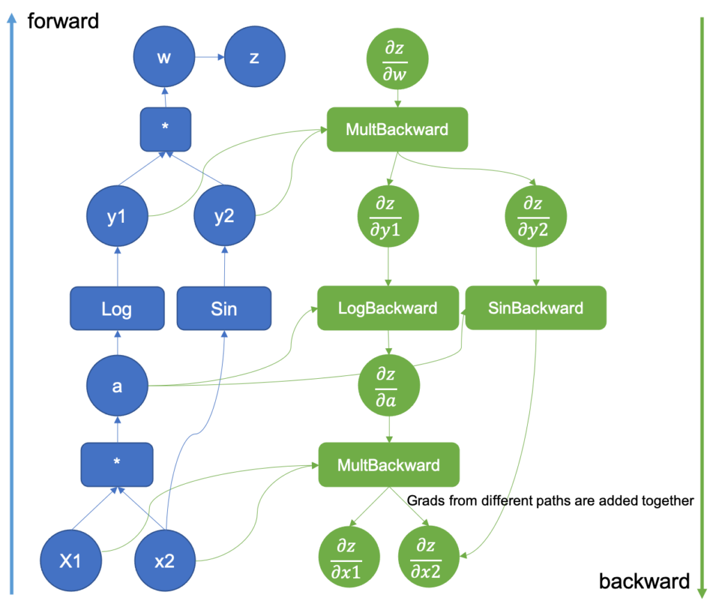
Backpropagation is not a separate kind of calculus. It is an efficient algorithm for applying the chain rule to a computational graph:

1. Run the forward pass, computing and caching intermediate values needed for local derivatives.
2. Start from the scalar loss, whose derivative with respect to itself is $1$.
3. Propagate derivative information backward through each operation.
4. At a point where the graph branches in the forward pass, sum gradient contributions from all downstream paths.

The last rule matters in networks with skip connections or any parameter reused in multiple computations. A parameter’s total gradient must capture every route by which changing it can change the loss.

---

A complete numerical gradient calculation

Take a single example with:

$$x=2$$ $$y=1$$ $$w=0.5$$ $$b=-1$$

The forward pass is:

$$z=wx+b=(0.5)(2)-1=0$$ $$\hat{y}=\sigma (0)=0.5$$ $$\ell =\frac{1}{2}(0.5-1{)}^2=0.125$$

Now work backward. First calculate the error signal at the pre-activation:

$$\delta =(\hat{y}-y)\hat{y}(1-\hat{y})$$ $$\delta =(0.5-1)(0.5)(1-0.5)=-0.125$$

Then calculate parameter gradients:

$$\frac{\partial \ell }{\partial w}=\delta x=(-0.125)(2)=-0.25$$ $$\frac{\partial \ell }{\partial b}=\delta =-0.125$$

The negative gradients mean that, at this point, increasing both $w$ and $b$ should reduce this example’s loss. This makes intuitive sense: the target is $1$, but the prediction is only $0.5$, so the model needs a larger logit $z$ and hence a larger predicted probability.

For a layer with vector input $\mathbf{x}$, output $\mathbf{z}$, weight matrix $W$, and bias vector $\mathbf{b}$:

$$\mathbf{z}=W\mathbf{x}+\mathbf{b}$$

Suppose:

$$W\in {\mathbb{R}}^{m\times d}$$ $$\mathbf{x}\in {\mathbb{R}}^{d\times 1}$$ $$\mathbf{z},\mathbf{b}\in {\mathbb{R}}^{m\times 1}$$

If the upstream gradient is:

$${\mathbf{g}}_z=\frac{\partial L}{\partial \mathbf{z}}\in {\mathbb{R}}^{m\times 1}$$

then the central backward-pass equations are:

$$\frac{\partial L}{\partial W}={\mathbf{g}}_z{\mathbf{x}}^T\in {\mathbb{R}}^{m\times d}$$ $$\frac{\partial L}{\partial \mathbf{b}}={\mathbf{g}}_z\in {\mathbb{R}}^{m\times 1}$$ $$\frac{\partial L}{\partial \mathbf{x}}=W^T{\mathbf{g}}_z\in {\mathbb{R}}^{d\times 1}$$

This is a useful dimension check from the previous lesson: the gradient of a parameter must have the same shape as that parameter. In particular, $\frac{\partial L}{\partial W}$ must have the same shape as $W$.

For a mini-batch $B$, training usually minimizes average loss:

$$L_B(\mathbf{\theta })=\frac{1}{|B|}\sum _{i\in B}{\ell }_i(\mathbf{\theta })$$

Thus, its gradient is the average of the per-example gradients:

$${\nabla }_{\mathbf{\theta }}{L}_B=\frac{1}{|B|}\sum _{i\in B}{\nabla }_{\mathbf{\theta }}{\ell }_i$$

Modern frameworks compute these vectorized quantities automatically, but the underlying calculation remains this repeated local application of the chain rule.

---

From gradients to parameter updates

Once backpropagation has produced a gradient, gradient descent chooses a parameter change in the opposite direction:

$${\mathbf{\theta }}_{t+1}={\mathbf{\theta }}_t-\eta {\nabla }_{\mathbf{\theta }}L({\mathbf{\theta }}_t)$$

The scalar $\eta >0$ is the learning rate.

Substitute the proposed change:

$$\mathbf{ϵ}=-\eta {\nabla }_{\mathbf{\theta }}L$$

into the first-order approximation:

$$L(\mathbf{\theta }+\mathbf{ϵ})\approx L(\mathbf{\theta })-\eta {\Vert {\nabla }_{\mathbf{\theta }}L\Vert }_2^2$$

For a sufficiently small learning rate, this predicted change is non-positive. That is why the negative gradient is the direction of steepest local decrease under the usual Euclidean geometry.

Returning to the numerical neuron example, use:

$$\eta =0.1$$

The update is:

$$w_{\text{new}}=0.5-0.1(-0.25)=0.525$$ $$b_{\text{new}}=-1-0.1(-0.125)=-0.9875$$

Both parameters increase, as predicted by the negative gradients. The new logit is:

$$z_{\text{new}}=(0.525)(2)-0.9875=0.0625$$

The new prediction is slightly above $0.5$, closer to the target $1$, and the loss falls.

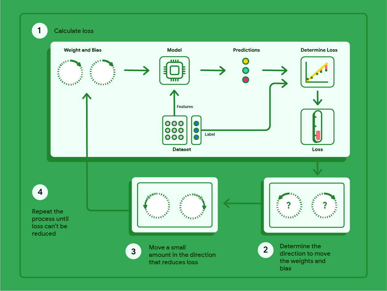
A practical training iteration therefore has four conceptual parts:

1. Forward pass: compute predictions from a mini-batch.
2. Loss computation: compare predictions with targets.
3. Backward pass: use backpropagation to compute parameter gradients.
4. Optimizer step: update parameters using the gradients and a learning-rate rule.

The terms are often conflated, so state them distinctly in interviews:

• Backpropagation computes gradients efficiently.
• Gradient descent uses gradients to update parameters.
• Automatic differentiation is the software mechanism that records operations and executes the backward calculations.
• An optimizer implements a particular update rule. Plain SGD is the simplest example.

---

What can go wrong, and how to validate gradients

The update equation is simple, but it is only a local approximation. Several implementation and optimization issues can make training fail.

Learning rate too large. The first-order approximation no longer predicts the true loss well across such a large step. Loss can oscillate, diverge, or become numerically invalid.

Learning rate too small. Loss may decrease, but impractically slowly. In a finite training budget, this can look like stalled learning.

Feature scale changes gradient scale. In the scalar example,

$$\frac{\partial \ell }{\partial w}=\delta x$$

Scaling $x$ by $1000$ scales the weight gradient by $1000$. This is one mathematical reason input normalization often makes optimization more stable.

Incorrect loss reduction. A common implementation bug is summing loss in one place and averaging it in another, changing gradient magnitude with batch size. If training behavior changes dramatically when only batch size changes, inspect loss reduction and learning-rate scaling.

Broken computational graph. Accidental detachment, incorrect tensor broadcasting, in-place mutation, or a non-differentiable operation can eliminate or corrupt a gradient. In a production training pipeline, logging gradient norms by layer and checking for missing gradients should be standard debugging steps.

For a small model or custom operation, use a finite-difference gradient check. For coordinate $i$, compare backpropagation’s derivative with:

$$\frac{\partial L}{\partial {\theta }_i}\approx \frac{L(\mathbf{\theta }+ϵ{\mathbf{e}}_i)-L(\mathbf{\theta }-ϵ{\mathbf{e}}_i)}{2ϵ}$$

where ${\mathbf{e}}_i$ changes only coordinate $i$. This is too expensive for routine large-model training, but it is highly effective for validating a new loss function or custom layer on a tiny deterministic example.

A precise interview response when asked why backpropagation is needed:

“A neural network is a composition of differentiable operations. Backpropagation applies the chain rule from the scalar loss backward through that computation graph, reusing intermediate values to compute the gradient with respect to every parameter efficiently. Gradient descent then subtracts a learning-rate-scaled version of that gradient. The negative sign matters because the gradient points toward the steepest local increase in loss.”

---

Key takeaways

A gradient is a vector of partial derivatives that describes local loss sensitivity to each parameter. The chain rule lets you compute a parameter gradient by multiplying local derivatives along a dependency path; when a value influences the loss by multiple paths, its contributions add.

Backpropagation is the reverse traversal that computes these gradients efficiently after a forward pass. For a simple sigmoid unit with squared loss:

$$\frac{\partial \ell }{\partial w}=(\hat{y}-y)\hat{y}(1-\hat{y})x$$ $$\frac{\partial \ell }{\partial b}=(\hat{y}-y)\hat{y}(1-\hat{y})$$

Gradient descent converts those gradients into learning:

$${\mathbf{\theta }}_{t+1}={\mathbf{\theta }}_t-\eta {\nabla }_{\mathbf{\theta }}L({\mathbf{\theta }}_t)$$

The backward pass computes sensitivities; the optimizer uses them to change parameters. Keeping that distinction clear will help in both deep-learning debugging and technical interviews.

Next, you will begin the Classical Machine Learning and Evaluation module by deriving linear-regression predictions and regularized training objectives.