Loss Functions: Regression vs. Classification

Welcome to the first lesson of our third module, Optimization and Model Fitting. In our previous work, we derived models like linear and logistic regression and even delved deep into the cross-entropy loss function from the perspective of Maximum Likelihood Estimation and information theory. We established that the goal of training is to find model parameters that minimize a chosen loss function.

In this lesson, we will generalize this concept. Our objective is to define and compare the most common loss functions used for both regression and classification tasks. We will explore the mathematical formulations and, more importantly, the theoretical properties of Mean Squared Error (MSE), Mean Absolute Error (MAE), and Cross-Entropy. Understanding their respective strengths and weaknesses is fundamental to the entire practice of model optimization. This exploration of what we optimize sets the stage perfectly for our next lesson, where we will discuss how we perform that optimization using gradient descent.

The Role of a Loss Function

At its core, a machine learning model is a function that maps inputs to outputs. The training process is about tuning the parameters of this function so that its outputs are as close as possible to the true, ground-truth values. A loss function, denoted as $L(\hat{y},y)$, provides a formal, quantitative measure of the "cost" or "error" incurred by a single prediction $\hat{y}$ when the true value is $y$.

The overall goal of training is to minimize the average loss over an entire dataset. This average is often called the cost function or empirical risk. The choice of loss function is not arbitrary; it is a crucial design decision that depends on the specific machine learning task.

To begin, let's get a formal overview of this concept from a recent review paper on the topic.

As the reading makes clear, loss functions are broadly categorized by task. Let's now examine the two primary families: those for regression and those for classification.

Loss Functions for Regression

In regression, the goal is to predict a continuous numerical value—for example, the price of a house or the temperature tomorrow. The loss, therefore, measures the distance between the predicted number and the true number.

Mean Squared Error (MSE)

The most common loss function for regression is the Mean Squared Error (MSE), also known as L2 Loss. Its origin lies in the method of Ordinary Least Squares (OLS), a cornerstone of classical statistics.

The MSE for a dataset of $N$ samples is defined as the average of the squared differences between the true values $y_i$ and the predicted values ${\hat{y}}_i$.

The key characteristic of MSE is the squaring of the error term $(y_i-{\hat{y}}_i)$. This has two important consequences:

1. Heavy penalty for large errors: A large error of 10 results in a loss of 100, whereas a small error of 0.1 results in a loss of only 0.01. This means the model is strongly incentivized to avoid large deviations.
2. Sensitivity to outliers: Because large errors are squared, a few outlier data points with significant errors can dominate the total loss, pulling the model fit disproportionately towards them.

Mean Absolute Error (MAE)

An alternative to MSE is the Mean Absolute Error (MAE), or L1 Loss. Instead of squaring the difference, it takes the absolute value.

By using the absolute value, the loss increases linearly with the error. This makes MAE significantly more robust to outliers compared to MSE. An error of 10 contributes 10 to the loss, and an error of 20 contributes 20. The penalty scales linearly, not quadratically.

Comparing MSE and MAE

The choice between MSE and MAE involves a trade-off between outlier sensitivity and optimization characteristics. The following video provides an excellent visual and intuitive comparison.

Let's visualize the shape of these loss functions.

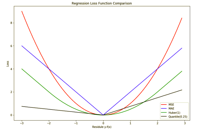
As the plot and video highlight, the key differences are:

• Sensitivity: MSE is highly sensitive to outliers due to its quadratic nature. MAE is more robust as it treats all errors with a consistent linear penalty.
• Optimization: MSE is a smooth, convex function that is differentiable everywhere. Its gradient is $2({\hat{y}}_i-y_i)$, which is straightforward to compute for optimization algorithms like gradient descent. MAE, on the other hand, is not differentiable at zero. This requires using techniques like sub-gradient descent, a detail your computer science background might find interesting, as it adds a slight complexity to the optimization algorithm.

If your problem's data contains significant outliers that you believe are anomalies (e.g., data entry errors), MAE might be a better choice. If large errors are genuinely critical and must be avoided at all costs, MSE's heavy penalization could be beneficial.

Loss Function for Classification

In the previous lesson, we took a deep dive into Cross-Entropy Loss, establishing its connection to Maximum Likelihood Estimation. For a classification problem with a probabilistic model (e.g., logistic regression or a neural network with a softmax output), we found that maximizing the log-likelihood of the data is equivalent to minimizing the negative log-likelihood.

The following video provides a concise and rigorous mathematical argument demonstrating that minimizing this negative log-likelihood is precisely the same as minimizing the cross-entropy between the model's predicted probability distribution and the true data distribution. This will solidify the theoretical foundation from our last lesson.

This equivalence is a cornerstone of modern classification models. It gives us a profound justification for our choice of loss function: training a classifier with cross-entropy is equivalent to finding the model parameters that make the observed labels most probable.

Let's quickly review the formula for cross-entropy from the appendix of our review paper.

Notice that the formula for Binary Cross-Entropy is exactly what we derived for logistic regression in the previous module. The more general Cross-Entropy Loss is what you would use for a multi-class problem, where $y_i$ is 1 for the true class and 0 for all others (one-hot encoding), effectively selecting only the log-probability of the correct class, $-\log ({\hat{y}}_{\text{true class}})$.

Comparing the Loss Functions: Why Not Use MSE for Classification?

We now have our standard choices: MSE for regression and Cross-Entropy for classification. A natural question arises: why can't we use MSE for a classification task? After all, in binary classification, the labels are 0 and 1, and the model outputs a probability between 0 and 1. We could certainly compute the squared difference.

The reason is twofold, relating to both the optimization landscape and the nature of the loss itself.

1. Vanishing Gradients and Non-Convexity: When using MSE with a sigmoid or softmax output, the resulting loss surface can become non-convex and plagued by "flat" regions. For instance, if the true label is 1 but the model confidently predicts 0 (so $\hat{y}$ is close to 0), the error is large. However, the derivative of the sigmoid function is very small at its extremes. The gradient of the MSE loss depends on this small derivative, causing the overall gradient signal sent back to the model to be tiny. This phenomenon, known as a vanishing gradient, means the model learns extremely slowly when it is most wrong.
2. Probabilistic Interpretation: Cross-entropy loss punishes confident, incorrect predictions exponentially. If the true class is 1, the loss is $-\log (\hat{y})$. As $\hat{y}\to 0$, the loss approaches infinity. This provides a very strong gradient signal, encouraging the model to correct its mistake quickly. Cross-entropy is fundamentally designed to measure the "distance" between two probability distributions, which is exactly what we are doing in classification. MSE simply measures numerical distance, ignoring this probabilistic structure.

This is a critical distinction that solidifies Cross-Entropy as the theoretically sound and practically superior choice for classification.

Conclusion

In this lesson, we formalized the concept of a loss function and compared the canonical choices for regression and classification. This understanding is essential for any practitioner, as the loss function defines the very objective of the learning process.

Here are the key takeaways:

• Loss functions quantify the error of a model's predictions and guide the optimization process. The choice is task-dependent.
• For regression, Mean Squared Error (MSE) is the default choice. It is differentiable and penalizes large errors heavily, but is sensitive to outliers. Mean Absolute Error (MAE) is an alternative that is more robust to outliers but has a discontinuous gradient.
• For classification, Cross-Entropy Loss is the standard. It is derived from the principle of Maximum Likelihood Estimation and has a deep connection to information theory. It correctly measures the dissimilarity between the predicted and true probability distributions and provides strong learning signals.
• Using a regression loss like MSE for a classification task is generally a poor choice due to potential optimization issues (vanishing gradients) and its lack of a proper probabilistic interpretation.

You have now defined the "what"—the objective to be minimized. In our next lesson, we will turn our attention to the "how" by exploring gradient descent, the fundamental iterative algorithm used to find the model parameters that minimize these loss functions.