Recommended resources
The freely available resources this lesson will direct you to.
Welcome back. Your step-count experiment treated the denoiser as a function you could call repeatedly. This final lesson opens that function call up and connects the objects in your Colab notebook to the notation used in masked-diffusion papers. The goal is practical: when you encounter a clean sequence, a noisy state, or a reverse update in an equation, you should know which tensor or operation it describes.
Start with the picture
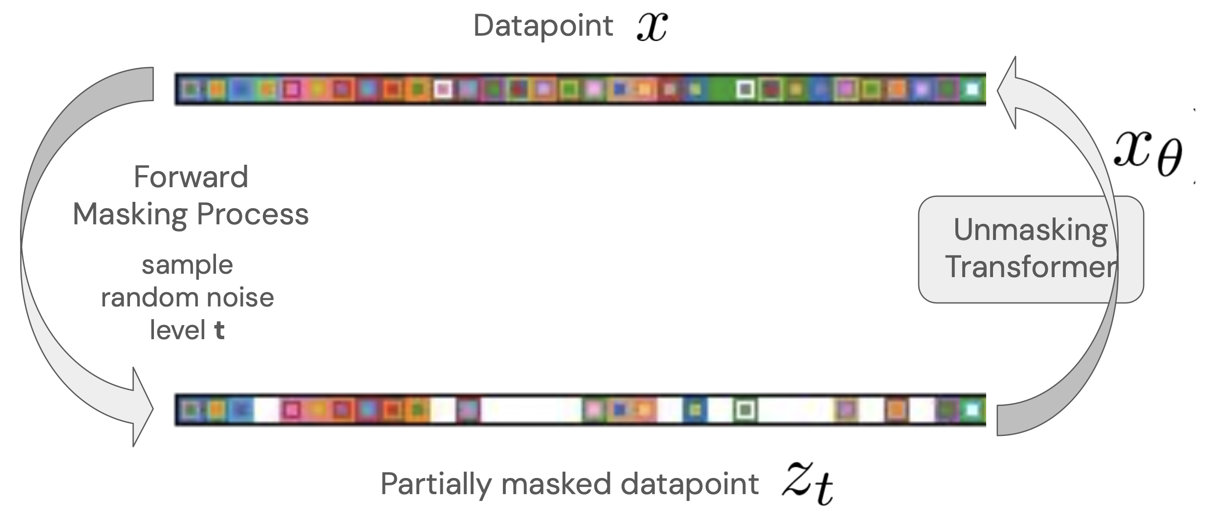
The distinction in the caption matters. During training, you have the clean sequence and can check the model’s predictions against it. During generation, you do not have the clean answer: you start with masks and construct an answer through reverse updates.
The Kuleshov Group’s How to Build a Diffusion Language Model gives a compact explanation of both situations.
How to Build a Diffusion Language Model | Kuleshov Group
Read the Kuleshov Group's explanation to connect the training picture to the reverse update used at generation time.
Under “Simple Masked Diffusion Models” → “Masked Diffusion in a Nutshell,” read the training idea. Then go to “Understanding Masked Diffusion: A Probabilistic Perspective” → “Reverse process.” Starting at the paragraph that derives the reverse process when the clean sequence is known, read the reverse explanation through the end of that paragraph. Focus on the substitution: at generation time, model predictions stand in for unknown clean tokens.
A paper-to-notebook dictionary
The following notation appears in the Section 3.1 excerpt of Not All Denoising Steps Are Equal. That is a different paper from the one you linked for this course. Use its definitions as a guide when reading your linked paper’s Section 3.1, but do not assume the two papers use identical symbols or identical samplers.
Not All Denoising Steps Are Equal: Model Scheduling for Faster Masked Diffusion Language Models
Read this paper's Section 3.1 for a concise research-paper statement of the objects you have implemented.
In “3 Accelerating MDLM via Model Scheduling” → “3.1 Experimental setup,” begin at “Masked diffusion language models.” Read from the clean-sequence definition, including the sentence that introduces the clean sequence. Continue through “Forward process,” especially pure masking and schedule; stop after the sentence about sampling the training time uniformly. Skip “Denoiser and training objective” for now. Under “Sampling (reverse process),” read the sampling description. Notice which tokens can change after an update.
Here is the translation for a batch of sequences, each stored at padded length , with vocabulary size :
| Paper concept | Meaning | Colab counterpart |
|---|---|---|
| Clean sequence | The original, uncorrupted tokens | clean_ids, integer IDs of shape [B, L] |
| Corrupted state | Clean tokens with some positions replaced by the mask symbol | corrupted_ids, also [B, L] |
| Noise level | How strongly the forward process corrupts a sequence | A value per batch row, commonly shape [B] |
| Denoiser | Predictions about original tokens given the current state | logits = denoiser(...), shape [B, L, V]; softmax gives per-position vocabulary distributions |
| Reverse state , where | A state with fewer masked positions | A copy of the current IDs with selected masks replaced by predicted token IDs |
A paper may denote the denoiser’s candidate clean tokens by or . In code, those are token IDs selected from the logits. They are not the clean training tensor clean_ids: during generation, that true answer is unavailable.
The paper’s usually counts sequence positions, whereas a notebook batch may contain padding. Your valid Boolean mask tells you which positions represent actual text. Padding is neither a clean text token to learn nor a blank to reveal.
Follow one training example
Suppose the clean sequence is c a t [PAD]. One possible corrupted sample is [MASK] a [MASK] [PAD]. The clean IDs are the target; the corrupted IDs are the denoiser’s input. The model predicts a distribution at every position, but your training loss checks only the two masked, valid positions.
With the linear schedule used in the Section 3.1 excerpt, : each valid token is retained with probability and masked with probability . If , masking two of the three valid characters is unsurprising, but not guaranteed. sets a probability, not an exact mask count.
The core tensor operation looks like this; the rest of your notebook already supplies clean_ids, valid, and MASK_ID:
# clean_ids: [B, L] integer token IDs
# valid:     [B, L] bool; False at padding positions
B, L = clean_ids.shape
t = torch.rand(B, device=clean_ids.device)             # [B]

masked = (torch.rand(B, L, device=clean_ids.device)
          < t[:, None]) & valid                         # [B, L]
corrupted_ids = torch.where(masked, MASK_ID, clean_ids) # z_t
The random comparison samples the forward corruption. It is not a learned prediction. Your loss uses clean_ids as targets and masked to select positions, with the safe empty-mask handling you implemented earlier.
Follow one generation update
Now remove clean_ids from the picture. For unconditional generation, begin with masks at every output position. The denoiser receives the current state , returns logits, and your sampler decides which predictions to keep. In the irreversible-commitment sampler you built, an update has this structure:
# z_t: current [B, L] token IDs
# valid: positions belonging to the output, not padding
# t: current per-row noise-level input, if your model uses one
logits = denoiser(z_t, t, valid)  # Adapt arguments to your module.
candidate_ids = logits.argmax(dim=-1)                  # [B, L]

still_masked = (z_t == MASK_ID) & valid
# reveal_now is a [B, L] bool mask chosen by your reveal schedule
# and, if used, confidence scores. It selects only still_masked positions.
z_s = torch.where(reveal_now, candidate_ids, z_t)
Your actual sampler may sample candidates rather than take argmax, and should exclude special symbols such as [PAD] and [MASK] from token candidates where appropriate. Neither choice changes what the variables mean. In the last line, positions not selected for revelation retain their previous values; an already revealed token stays fixed in this sampler. With an optional fixed prefix, its positions likewise remain unchanged.
The Kuleshov Group’s reverse-process explanation describes a probabilistic rule for choosing which masks to uncover. Your confidence-ranked reveal_now is a sampler choice, not that exact probabilistic rule. Both use a denoiser prediction to make a less-masked state, but you should not equate their update probabilities. Likewise, a requested next noise level describes the schedule; a finite sequence’s realized masked fraction need not equal exactly.
When you read the linked paper’s Section 3.1, identify each object by its role rather than its letter: Which variable is the known training text? Which is the partially masked input? Is its time parameter a masking probability or a retention probability? Does the model output vocabulary distributions or selected token IDs? Finally, does its reverse rule randomly reveal tokens, rank them by confidence, or permit remasking? Those answers determine how closely each equation matches your Colab operations.
Takeaways
You can now read the central masked-diffusion story as tensor operations: clean_ids supplies training targets; a noise level controls random masking to produce corrupted_ids; the denoiser produces vocabulary logits; and a sampler uses selected predictions to update the masked state. The most important boundary is that clean text is known during training but must be predicted during generation.
That closes the course’s path from first principles to a working mini diffusion language model. Your notebook is also a useful reference when a larger paper changes notation—or uses a reverse-update policy different from yours.