Kadanoff Block-Spin Renormalization for 1D Ising Model

Recommended resources

The freely available resources this lesson will direct you to.

Hello! Welcome to your second lesson on the renormalization group.

In our previous lesson, we established the physical motivation for the RG framework. We saw that the scale invariance of a system at its critical point is the central challenge, and that the RG addresses this through a two-step process of coarse-graining and rescaling. This process generates a flow in the space of Hamiltonian parameters, where critical points correspond to fixed points of this flow.

Today, we will move from the conceptual to the concrete. Our goal is to apply this machinery to our favorite toy system: the one-dimensional Ising model. You will learn how to perform a specific type of real-space RG called decimation, which is a simple and elegant form of the Kadanoff transformation. By explicitly carrying out this procedure, we will derive the RG flow equation for the 1D Ising model and use it to rigorously demonstrate the absence of a phase transition at any finite temperature.

The Real-Space RG for the 1D Ising Model

To begin, we need a Hamiltonian that is general enough to be preserved under the RG transformation. If we start with just the nearest-neighbor coupling $J$ , the coarse-graining step will generate new terms. To create a "closed" system, we must start with the most general nearest-neighbor Hamiltonian for a 1D chain of N spins $σ_{i} = \pm 1$ :

- β H = i = 1 \sum N (g + \frac{h}{2} (σ_{i} + σ_{i + 1}) + K σ_{i} σ_{i + 1})

Here, $K = β J$ is the dimensionless coupling, $h$ is the dimensionless external field, and $g$ is a spin-independent constant that tracks the contribution to the free energy from the integrated-out degrees of freedom. We've written the field term symmetrically over the bond connecting sites $i$ and $i + 1$ .

The partition function is $Z_{N} = Tr (e^{- β H})$ . Our task is to perform a partial trace over some of the spins and show that the resulting partition function describes a new Ising chain with renormalized parameters $g^{'}, h^{'}, K^{'}$ .

The specific coarse-graining procedure we'll use is decimation, which simply means summing over every other spin. For example, we will sum over all even-numbered spins ( $σ_{2}, σ_{4}, \dots$ ), leaving an effective model for the odd-numbered spins. This is a simple implementation of Kadanoff's idea: we are effectively creating "blocks" of two spins and letting the odd-numbered spin represent the block.

Deriving the Recursion Relations

The core of the lesson is the derivation of the mapping $(g, h, K) \to (g^{'}, h^{'}, K^{'})$ . This mapping defines the RG flow. The calculation is detailed and algebraically intensive, making it a perfect exercise for seeing the theory in action.

13. Position Space Renormalization Group, Part 1

The following lecture by Prof. Mehran Kardar provides a masterclass in this derivation. It is clear, rigorous, and directly aligned with our goal. We will watch it in two parts.

First, watch from 19:52 to 26:51. This section sets up the problem, introduces the 1D Ising chain, and explains the decimation procedure of 'getting rid of every other spin.' Next, watch the detailed derivation from 26:51 to 45:46. This is the heart of the calculation. Focus on: How the partition function is rewritten to isolate the sums over the 'even' spins. The summation over a single spin 's' sandwiched between two 'prime' spins that are being kept. The crucial step of matching the result of this sum to the form of the new Hamiltonian to find the new parameters. Prof. Kardar uses the variables x, y, z for e^K, e^h, e^g, which greatly simplifies the algebra.

The RG Flow Equations

After watching the derivation, let's consolidate the results. The process of summing over an intermediate spin $σ_{2 i}$ between two remaining spins $σ_{2 i - 1}^{'}$ and $σ_{2 i + 1}^{'}$ leads to the following relation:

σ_{2 i} = \pm 1 \sum exp [B (σ_{2 i - 1}^{'}, σ_{2 i}) + B (σ_{2 i}, σ_{2 i + 1}^{'})] = exp [2 g^{'} + B^{'} (σ_{2 i - 1}^{'}, σ_{2 i + 1}^{'})]

Here, $B$ represents the terms inside the sum in our original Hamiltonian for a single bond, and $B^{'}$ represents the term for the new effective bond. The factor of $2 g^{'}$ arises because integrating out one spin $σ_{2 i}$ contributes to the free energy associated with the two new bonds it helps create (one to its left, one to its right).

By explicitly evaluating the sum for the four possible configurations of $(σ_{2 i - 1}^{'}, σ_{2 i + 1}^{'})$ , as shown in the video, one arrives at a set of three equations relating the new parameters to the old. While the full equations for $K^{'}, h^{'}, g^{'}$ are complex, let's focus on the physically most interesting case: zero external field ( $h = 0$ ).

The Zero-Field Case ( $h = 0$ )

When $h = 0$ , the system has up-down symmetry ( $σ \to - σ$ ). An RG transformation should preserve this symmetry, so we expect that if we start with $h = 0$ , we will have $h^{'} = 0$ . The equations from the video confirm this: setting $y = e^{h} = 1$ gives $y^{'} = e^{h^{'}} = 1$ .

The recursion relations simplify significantly. The core equation for the coupling $K$ becomes:

e^{2 K^{'}} = cosh (2 K)

K^{'} = \frac{1}{2} ln (cosh (2 K))

The constant term $g$ evolves according to:

e^{4 g^{'}} = 4 cosh^{2} (2 K) e^{4 g} ⟹ g^{'} = g + \frac{1}{2} ln (2 cosh (2 K))

This $g^{'}$ term tracks the accumulating free energy, but the critical behavior is governed entirely by the flow of the coupling constant $K$ .

[PDF] 7.3 The Renormalization Group

The derivation for the zero-field case is fundamental. To see it again in a concise, textbook format, please read the following section from Franz Schwabl's 'Statistical Mechanics'.

Read the subsection '7.3.2 The One-Dimensional Ising Model, Decimation Transformation'. It re-derives the recursion relations for K' and g in the zero-field case, which should be a good reinforcement of the video's content.

Analysis of the Flow and Fixed Points

The equation $K^{'} = \frac{1}{2} ln (cosh (2 K))$ is the RG flow equation for the 1D Ising model at zero field. It tells us how the effective coupling constant changes as we view the system at larger and larger scales (each step corresponds to a doubling of the length scale).

To understand the long-distance physics, we look for the fixed points of this flow, where $K^{*} = K^{'}$ .

K^{*} = \frac{1}{2} ln (cosh (2 K^{*}))

By inspection or graphical analysis, this equation has two solutions:

$K^{*} = 0$ : This is the high-temperature fixed point. At infinite temperature, $J = 0$ , so $K = 0$ . The spins are completely uncorrelated.
$K^{*} = \infty$ : This is the zero-temperature fixed point. At $T = 0$ , the coupling is infinite, and the system is perfectly ordered.

Now, we must analyze the stability of these fixed points by examining the flow nearby.

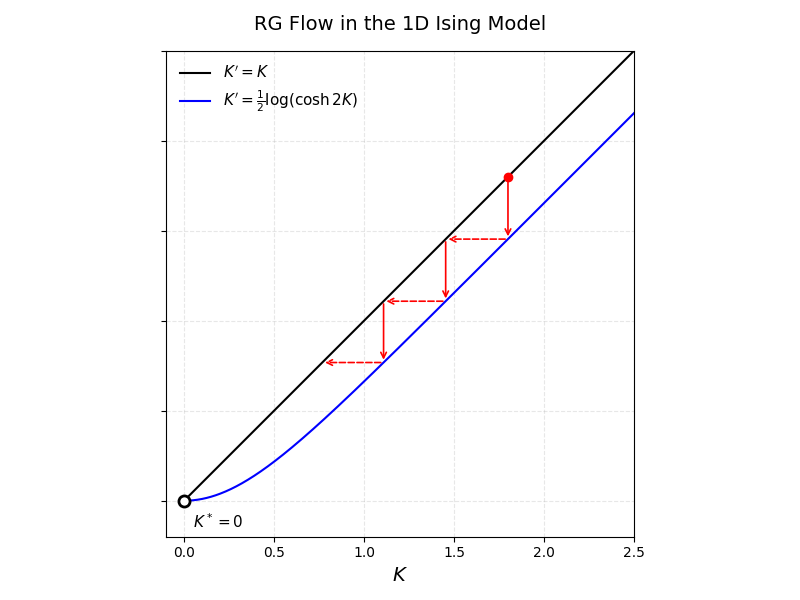
RG Flow in the 1D Ising Model — This diagram illustrates the RG flow for the coupling K. The transformation K' = f(K) is plotted in blue, and the identity line K' = K is in black. The arrows show that for any initial value K > 0, repeated applications of the RG transformation cause the coupling to flow towards the stable fixed point at K* = 0.

As the diagram shows:

Near $K = 0$ : We can expand $cosh (2 K) \approx 1 + \frac{( 2 K ) ^{2}}{2} = 1 + 2 K^{2}$ . Then, using $ln (1 + x) \approx x$ , we get $K^{'} \approx \frac{1}{2} (2 K^{2}) = K^{2}$ . Since $K^{2} < K$ for small $K$ , the flow is directed towards $K = 0$ . This is a stable fixed point.
Near $K = \infty$ : We can approximate $cosh (2 K) \approx \frac{1}{2} e^{2 K}$ . The flow equation becomes $K^{'} \approx \frac{1}{2} ln (\frac{1}{2} e^{2 K}) = K - \frac{1}{2} ln 2$ . Since $K^{'} < K$ , the flow is directed away from $K = \infty$ . This is an unstable fixed point.

The physical implication is profound. If you start with any finite coupling $K > 0$ (i.e., any finite temperature $T$ ), the RG flow will always drive your system towards the $K = 0$ disordered fixed point. A finite-temperature phase transition would require an unstable fixed point at a finite $K_{c} > 0$ . The absence of such a fixed point is a rigorous proof that the 1D Ising model does not have a phase transition at any finite temperature. The only "critical" behavior occurs at the unstable fixed point $T = 0$ .

Test your understanding!

In our analysis, the term $g$ evolved as $g^{'} = g + \frac{1}{2} ln (2 cosh (2 K))$ . Why can we ignore this flow equation when searching for critical points and analyzing their stability?

Show answer

The parameter $g$ is a spin-independent constant in the Hamiltonian. It shifts the overall energy of every configuration by the same amount and thus contributes a constant factor to the partition function, $Z \to Z \times e^{N g}$ . This affects the absolute value of the free energy per site ( $f \to f - k T g$ ) but does not alter any of its derivatives with respect to temperature or field.

Crucially, the flow equations for the physically relevant parameters, $K$ and $h$ , do not depend on $g$ . The relative probabilities of different spin configurations, which determine the ordering and response functions, are independent of $g$ . Therefore, the search for fixed points in the $(K, h)$ parameter space and the analysis of flows around them—which is what determines critical behavior—can be done without considering the flow of $g$ .

Conclusion

In this lesson, we have put the abstract concepts of the renormalization group into practice. By performing a decimation transformation on the 1D Ising model, we successfully derived its RG flow equations.

Key Takeaways:

Decimation is a simple real-space RG scheme where alternate degrees of freedom are integrated out (summed over).
To keep the Hamiltonian's form invariant, one must start with a general form that includes all terms generated by the RG transformation (in this case, $g, h, K$ ).
The derived RG flow equation for the coupling, $K^{'} = \frac{1}{2} ln (cosh (2 K))$ , dictates how the system behaves at progressively larger length scales.
The analysis of this flow reveals only two fixed points: a stable one at $K^{*} = 0$ ( $T = \infty$ ) and an unstable one at $K^{*} = \infty$ ( $T = 0$ ).
The absence of an unstable fixed point at a finite, non-zero coupling proves that the 1D Ising model cannot sustain long-range order at any $T > 0$ .

Preview of the Next Lesson:

We have now seen a complete, albeit simple, RG calculation. In the next lesson, we will step back and formalize the concepts we've used. We will define RG flows, fixed points, and their stability more generally, and classify fixed points to build a complete picture of how the RG framework explains the structure of phase diagrams and the universality of critical phenomena.