Classifying and Interpreting Fixed Points

Recommended resources

The freely available resources this lesson will direct you to.

Hello! Welcome back to our study of the Renormalization Group.

In our last lesson, we uncovered the mathematical engine of the RG: linearization. We saw that by analyzing the RG flow in the infinitesimal neighborhood of a fixed point $S^{*}$ , the transformation simplifies to a matrix equation $δ S^{'} = M \cdot δ S$ . The eigenvalues of this matrix, expressed as $λ_{i} = b^{y_{i}}$ , gave us the crucial RG exponents $y_{i}$ . We established that the sign of $y_{i}$ determines if a perturbation is relevant ( $y_{i} > 0$ ), irrelevant ( $y_{i} < 0$ ), or marginal ( $y_{i} = 0$ ). We also derived the profound connection between these exponents and the measurable critical exponents like $ν$ .

Today, we will use this framework to build a complete picture of the RG flow diagram. Our objective is to formally classify fixed points as stable, unstable, or marginal and interpret their physical meaning. By understanding the nature of these special points, we can understand the global structure of phase diagrams and the principle of universality.

The Classification of Fixed Points

The stability of a fixed point is entirely determined by the set of RG exponents ${y_{i}}$ associated with it. These exponents are the eigenvalues of the linearized flow matrix, as you learned previously. Let's formalize the classification.

To start, let's review the core idea from a concise text.

[PDF] Renormalization Group Flow Near the Trivial Fixed Point

The following resource provides a very clear and formal definition of fixed points and the classification of perturbations as relevant or irrelevant based on the eigenvalues of the linearized flow.

Please read Section 7, 'Fixed points and (ir)relevant directions'. This section defines a fixed point in the context of RG flow equations and explains how linearizing the flow around it allows you to classify perturbations as relevant or irrelevant based on the sign of the eigenvalues of the matrix M.

Based on this, we can define three types of fixed points:

1. Unstable Fixed Points

Definition: An unstable fixed point has at least one relevant operator (i.e., at least one $y_{i} > 0$ ).
RG Flow: The flow trajectories move away from the fixed point along the directions of the relevant eigenvectors. Trajectories may be attracted towards it along irrelevant directions. In the language of dynamical systems, this type of fixed point is often a saddle point.
Physical Interpretation: An unstable fixed point represents a critical point. Its correlation length is infinite ( $ξ^{*} = \infty$ ). The set of all points in parameter space that flow into the unstable fixed point forms the critical surface (or critical manifold). To land on this critical point, one must precisely tune the experimental parameters (like temperature) to lie on this surface. Any infinitesimal perturbation along a relevant direction will cause the system to flow away from criticality towards a stable phase. The number of relevant operators dictates the number of parameters you need to tune to achieve criticality. For a standard thermal phase transition, these are typically the temperature $t$ and the ordering field $h$ .

2. Stable Fixed Points

Definition: A stable fixed point has only irrelevant operators (i.e., all $y_{i} < 0$ ).
RG Flow: The flow trajectories move towards the fixed point from all directions in its vicinity. It acts as a "sink" for the RG flow. The set of all points that flow into it is called its basin of attraction.
Physical Interpretation: A stable fixed point represents a stable thermodynamic phase. The correlation length at such a point is zero ( $ξ^{*} = 0$ ). These correspond to states of complete order (like a ferromagnet at T=0) or complete disorder (like a paramagnet at T=∞). Any system starting within the basin of attraction of a stable fixed point will, upon repeated coarse-graining, look like the simple, scale-invariant state described by that fixed point.

3. Marginal Fixed Points

Definition: A fixed point with one or more marginal operators ( $y_{i} = 0$ ) and no relevant operators.
RG Flow: At the linear level, the flow does not move along the marginal direction. The ultimate direction of the flow (towards or away from the fixed point) is determined by higher-order, non-linear terms in the RG equations. A marginal operator may turn out to be marginally relevant or marginally irrelevant.
Physical Interpretation: These are more subtle and lead to interesting physics. They can indicate a line of fixed points, leading to critical behaviour over a range of parameters (as in the Kosterlitz-Thouless transition), or they can produce logarithmic corrections to the standard power-law scaling behaviour. The $ϕ^{4}$ theory at its upper critical dimension, $d = 4$ , is a key example where the coupling constant is a marginal operator.

The RG Flow Diagram: A Global Perspective

The classification of fixed points allows us to sketch the entire landscape of the RG flow. This diagram is essentially a map of the system's phase diagram.

The following resource provides an excellent discussion and a schematic diagram illustrating these concepts.

[PDF] Chapter 4 Renormalisation Group - TCM

To see how these different types of fixed points fit together to form a phase diagram, let's look at another excellent text.

Please read the text from the start of Section 4.2 'Formal Approach' up to the paragraph before Section 4.3 (pages 47-49). Pay close attention to Figure 4.2 and its caption. This section beautifully explains how an unstable fixed point with one relevant operator corresponds to a critical point, and its 'basin of attraction' (the critical surface) has codimension one. This explains universality: many different microscopic Hamiltonians (points in the parameter space) flow to the same critical fixed point and thus share the same critical exponents.

Let's look at a concrete, albeit approximate, example for the 2D Ising model.

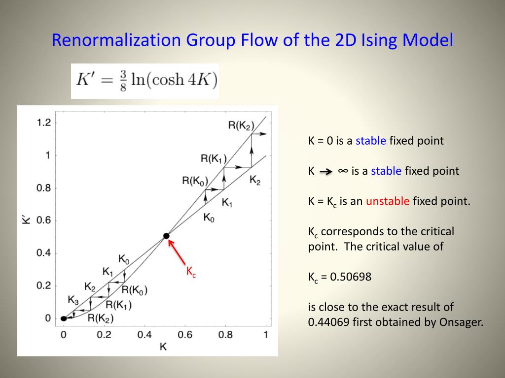
Renormalization Group Flow and Fixed Points for the 2D Ising Model — This image shows the RG flow for a single coupling K in an approximate 2D Ising model. The recursion relation K' = f(K) is plotted along with the line K' = K. The intersections are the fixed points.

In this diagram, we can clearly identify:

K=0 (T=∞): This is a stable fixed point. If you start with any small K (high temperature), the flow drives you towards K=0. This is the disordered paramagnetic phase.
K=∞ (T=0): This is another stable fixed point. If you start with a large K (low temperature), the flow drives you to even larger K. This is the ordered ferromagnetic phase.
K = Kc ≈ 0.507: This is an unstable fixed point. If you start slightly away from Kc, the flow pushes you away, either towards the disordered (K=0) or the ordered (K=∞) fixed point. This point represents the critical point of the phase transition.

An Analogy to Dynamical Systems

Given your background in mathematics, you'll recognize that this classification scheme is identical to the stability analysis of fixed points in systems of ordinary differential equations (ODEs). The RG flow equations, often written in differential form as $\frac{d g}{d ℓ} = β (g)$ , constitute a dynamical system.

A fixed point $g^{*}$ is where the "velocity" is zero: $β (g^{*}) = 0$ .
The linearized flow matrix $M$ is the Jacobian of the beta functions: $M_{ij} = \frac{\partial β _{i}}{\partial g _{j}}_{g^{*}}$ .
The RG exponents $y_{i}$ are the eigenvalues of this Jacobian.

Therefore:

A stable fixed point (all $y_{i} < 0$ ) is a sink or stable node.
An unstable fixed point in RG is typically a saddle point in the parameter space. It is attractive along irrelevant directions (forming the stable manifold, our critical surface) and repulsive along relevant directions (the unstable manifold).

The following video provides an excellent overview of this classification for general 2D systems. While the context is not RG specifically, the mathematical principles and the phase portraits are directly analogous.

Classifying Fixed Points of 2D Systems - Linear Stability Analysis

To solidify the connection to dynamical systems, watch these segments on classifying fixed points of 2D ODEs. Notice how the phase portraits of nodes and saddles look exactly like the RG flow diagrams we've been discussing.

Please watch the following clips from 'Classifying Fixed Points of 2D Systems': Nodes and Saddles (7:55 - 14:24): This part explains stable nodes (sinks), unstable nodes (sources), and saddle points based on the signs of the real eigenvalues. Pay attention to the phase portrait for the saddle point and compare it to the flow around a critical point. The Delta-Tau Plane (19:28 - 22:16): This provides a fantastic summary, classifying all possible fixed points in a 2D plane based on the trace (τ) and determinant (Δ) of the Jacobian matrix. Since the eigenvalues λ are roots of λ² - τλ + Δ = 0, this plane maps out all stability behaviors. A saddle point, corresponding to our critical point, occurs when Δ < 0 (λ₁ > 0, λ₂ < 0).

Test your understanding!

A certain phase transition is described by a theory with a three-dimensional parameter space $(g_{1}, g_{2}, g_{3})$ . An RG analysis reveals a fixed point at $g^{*} = (g_{1}^{*}, g_{2}^{*}, g_{3}^{*})$ . The linearized flow matrix $M$ at this fixed point has eigenvalues $y_{1} = 1.6$ , $y_{2} = - 0.8$ , and $y_{3} = - 2.1$ .

Classify this fixed point.
What is its physical significance?
What is the dimension of the critical surface associated with this fixed point?

Show answer

Classification: The fixed point has one positive eigenvalue ( $y_{1} > 0$ ) and two negative eigenvalues ( $y_{2} < 0, y_{3} < 0$ ). It has one relevant operator and two irrelevant operators. Therefore, it is an unstable fixed point (specifically, a saddle point).
Physical Significance: It represents a critical point. The system will only exhibit critical phenomena if its parameters are tuned to lie on the surface that flows into this fixed point. The single relevant operator likely corresponds to temperature, meaning this is a standard critical point reached by tuning one experimental parameter.
Dimension of the Critical Surface: The critical surface is the stable manifold of the unstable fixed point, spanned by the eigenvectors of the irrelevant operators. Since there are two irrelevant operators, the critical surface is two-dimensional. It is a surface of codimension 1 in the three-dimensional parameter space.

Conclusion

Today we have assembled a complete conceptual framework for understanding RG flow diagrams. By linearizing the flow around fixed points, we can classify them and assign them a clear physical meaning, revealing the deep connection between the topology of the flow and the structure of the phase diagram.

Key Takeaways:

Stable Fixed Points: Have only irrelevant operators ( $y_{i} < 0$ ), act as sinks in the RG flow, and represent stable thermodynamic phases (e.g., T=0 ordered, T=∞ disordered).
Unstable Fixed Points: Have one or more relevant operators ( $y_{i} > 0$ ), act as saddle points in the flow, and represent critical points.
Marginal Fixed Points: Have operators with $y_{i} = 0$ , requiring non-linear analysis, and can lead to more exotic critical phenomena.
The critical surface is the basin of attraction of an unstable (critical) fixed point. Its dimension is determined by the number of irrelevant operators.
Universality arises because many different physical systems (different points in parameter space) can lie in the basin of attraction of the same critical fixed point, thus sharing its universal critical properties.

Preview of the Next Lesson:

We have spent several lessons building up the conceptual and mathematical machinery of the RG. Now it's time to put it all into practice with a hands-on calculation. In the next lesson, we will perform a real-space RG calculation for the 2D Ising model on a square lattice using the decimation method. We will derive the recursion relations, find the fixed points, and analyze the resulting flow diagram ourselves.