Dissecting 3D Gaussian Splatting: Problem, Method, and Results

In our previous lesson, we established the critical trade-offs between the implicit, ray-marched world of NeRF and the explicit, rasterized universe of 3D Gaussian Splatting. You now possess the high-level context to appreciate not just what 3DGS does, but why its design was so revolutionary.

Now, we move from the summary to the source. This lesson marks our first formal application of your requested research decomposition framework. We will take the original paper, "3D Gaussian Splatting for Real-Time Radiance Field Rendering," and dismantle it into its three core pillars: the problem it confronts, the method it proposes, and the results that validate its claims. This is the fundamental skill of a research scientist—the ability to look past the dense equations and prose to see the clear, logical structure of an academic contribution.

Let's begin our analysis.

The Problem Statement

Every significant research paper begins by identifying a clear and compelling problem. A great paper doesn't just present a solution; it first convinces you that the problem is worth solving. For 3DGS, the authors identified a fundamental "trilemma" in the field of novel view synthesis.

Previous methods forced a choice between three desirable properties:

1. High Visual Quality: Achieving photorealistic results comparable to the best offline methods.
2. Fast Training Times: Creating the scene representation in minutes, not hours or days.
3. Real-Time Rendering: Synthesizing new views at interactive frame rates (e.g., >30 FPS).

Before 3DGS, no single method could deliver all three. Methods like Mip-NeRF360 achieved state-of-the-art quality but took up to 48 hours to train and were extremely slow to render. Faster methods like Instant-NGP or Plenoxels sacrificed significant visual quality to achieve faster training and interactive (but not truly real-time) rendering.

The authors of 3DGS explicitly state their goal is to break this trade-off. Let's read their own words from the paper's abstract.

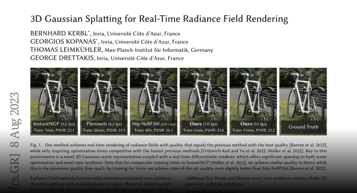
With the problem clearly defined as resolving this quality-speed trilemma, we can now dissect the technical machinery they built to solve it.

The Core Method

This is the heart of the paper, detailing the "how." We'll break it down into the mathematical representation and the architectural innovations that bring it to life, a structure that aligns perfectly with your interest in both first principles and high-performance systems engineering.

1. Mathematical and Representational Core

The foundational choice was to abandon the implicit MLP of NeRF in favor of an explicit representation using 3D Gaussians.

A 3D Gaussian is defined by a center (mean) $\mathbf{\mu }$ and a 3D covariance matrix $\mathbf{\Sigma }$.

These primitives were chosen because they are differentiable and can be analytically projected onto a 2D image plane, forming 2D "splats." This avoids the costly point-sampling of ray marching.

The full scene is represented by a set of these Gaussians, each with the following learnable parameters:

• Position ($\mathbf{\mu }$): A 3D vector for its location.
• Covariance ($\mathbf{\Sigma }$): A 3x3 matrix defining its shape and orientation. To make this optimizable, it's decomposed into a 3D scaling vector $\mathbf{s}$ and a rotation quaternion $\mathbf{q}$. This ensures the covariance matrix remains valid (positive semi-definite) during gradient-based optimization.
• Color ($\mathbf{c}$): Represented by Spherical Harmonics (SH) coefficients. This allows the color to be view-dependent, capturing effects like reflections.
• Opacity ($\alpha$): A scalar value controlling its transparency.

To better understand this representation and its projection, the LearnOpenCV article provides an excellent, more pedagogical walkthrough.

2. Architectural and Systems Innovation

Having an explicit representation is only half the story. The true genius of 3DGS lies in the systems designed to optimize and render these millions of Gaussians in real time. This is where the low-level engineering brilliance shines.

The method consists of two interleaved processes: optimization with adaptive density control and a fast, differentiable rasterizer.

For a concise video overview of the entire pipeline, watch this review.

Now let's break down those components using the original paper.

A. Optimization and Adaptive Density Control

The process starts with a sparse point cloud from Structure-from-Motion (SfM). These points are used to initialize the first set of Gaussians. The system then iteratively renders images, compares them to the ground truth training images using a loss function ($L_1+\lambda D\text{-SSIM}$), and updates the Gaussian parameters via stochastic gradient descent.

Crucially, the set of Gaussians is not static. The authors introduce an adaptive density control mechanism that dynamically adds and removes Gaussians to better fit the scene geometry.

• Densification: In areas where the rendered image doesn't match the ground truth well (indicated by large positional gradients), the system densifies the Gaussians.
  • For under-reconstruction (missing details), it clones small Gaussians to fill the space.
  • For over-reconstruction (blurry details from one large Gaussian), it splits the large Gaussian into two smaller ones.
• Pruning: Gaussians that become nearly transparent (very low $\alpha$) are periodically removed.

This process allows the model to "carve out" the scene's geometry, starting sparse and becoming dense only where needed.

B. The Fast Differentiable Rasterizer

This is the engine that enables real-time performance. Instead of ray marching, 3DGS uses a highly optimized rasterization pipeline inspired by traditional computer graphics but made fully differentiable.

The key steps, which you'll recognize from our previous lesson, are:

1. Culling: Discard Gaussians outside the camera's view frustum.
2. Projection: Project all 3D Gaussians to 2D splats on the screen.
3. Tiling: Divide the screen into 16x16 tiles.
4. Sorting: This is a major innovation. All Gaussians are sorted globally in a single pass using a highly efficient GPU radix sort. Each Gaussian is assigned a key based on its view-space depth and the tiles it overlaps. This avoids slow per-pixel sorting.
5. Rasterization: For each tile, threads collaboratively load the sorted Gaussians and blend them front-to-back for each pixel until the pixel is opaque. The backward pass for gradient computation cleverly re-uses the sorted list.

This entire pipeline was designed to maximize GPU parallelism and memory access patterns, a detail that someone with your systems programming interest can truly appreciate. It's a testament to the power of building algorithms that respect the underlying hardware architecture.

The Key Results

With the problem and method established, the final part of a paper is to present evidence that the method actually works. This is done through quantitative metrics, qualitative comparisons, and ablation studies.

Quantitative and Qualitative Comparison:
The authors compare their method against the leading competitors on several standard datasets. The main results (summarized in Table 1 of the paper) show that 3DGS achieves:

• Quality (PSNR/SSIM) on par with or slightly better than the previous state-of-the-art, Mip-NeRF360.
• Training times of ~40 minutes, comparable to fast methods like Instant-NGP and orders of magnitude faster than Mip-NeRF360 (48 hours).
• Rendering speeds of >100 FPS at 1080p, achieving true real-time performance where all others fall short.

Ablation Studies:
To prove that each part of their complex system is necessary, the authors perform ablation studies where they disable key components one by one and show that performance degrades. This is a hallmark of rigorous research.

One of the most telling ablations is the "Limited-BW" test, where they limit the number of Gaussians that receive gradients during backpropagation (a common practice in prior work). The quality plummets, proving the necessity of their efficient rasterizer that can backpropagate through an arbitrary number of primitives.

Conclusion

By systematically decomposing the paper, we have distilled its core contribution. You are no longer just a reader; you are an analyst who can articulate the paper's argument with precision.

Key Takeaways from the Decomposition:

• Problem: To resolve the trilemma in novel view synthesis by creating a method that is simultaneously high-quality, fast to train, and renders in real-time.
• Core Method: A novel combination of an explicit scene representation using anisotropic 3D Gaussians with a highly optimized, tile-based differentiable rasterizer. The method is brought to life by an adaptive density control scheme that dynamically refines the Gaussians during optimization.
• Key Results: The paper demonstrates through extensive experiments that 3DGS successfully achieves the goal, matching or exceeding the quality of the best previous methods while being orders of magnitude faster to train and render. Ablation studies confirm that each component of their proposed method is critical to its success.

This structured analysis gives you a powerful template for dissecting any research paper you encounter.

Preview of the Next Lesson:

A good researcher doesn't just understand a paper; they critique it. The final step in our analysis is to identify the limitations of 3D Gaussian Splatting. What can't it do? Where does it still struggle? Answering these questions is the first step toward formulating a novel research project. In our next lesson, we will put on our critic hats, analyze the paper's own "Limitations" section, and brainstorm potential follow-up research questions.