Adiabatic Theorem and Slowly Varying Hamiltonians

Hello! Welcome to our next lesson in quantum dynamics.

In our last session, we explored how a system responds to a harmonic perturbation, like an oscillating electromagnetic field. We found that such perturbations efficiently drive transitions between energy levels, and we quantified the rate using Fermi's Golden Rule.

Today, we will investigate the opposite extreme: what happens when a Hamiltonian changes not rapidly or periodically, but very, very slowly? This leads us to one of the most profound concepts in quantum mechanics: the adiabatic theorem. Our goal is to understand the conditions under which a quantum system can adapt to a changing environment without making transitions, and to analyze the subtle phase it acquires during this process. This principle is not just a theoretical curiosity; it underpins fundamental approximations in molecular and condensed matter physics.

1. Intuition and Statement of the Adiabatic Theorem

Before diving into the quantum mechanical details, it's helpful to build some intuition from classical mechanics. Your physics background will make this analogy quite natural.

As the reading shows, for a classical oscillator, if you slowly change the stiffness of the spring (and thus $\omega$), the energy $E$ will change, but the ratio $I=E/\omega$ remains nearly constant. This quantity $I$ is an adiabatic invariant.

In quantum mechanics, the energy of a harmonic oscillator is quantized: $E_n=\hslash \omega (n+1/2)$. The ratio $E_n/\omega$ is thus $\hslash (n+1/2)$. If we demand that $E/\omega$ be the invariant quantity, this implies that the quantum number $n$ does not change during the slow evolution.

This is the heart of the quantum adiabatic theorem: if a system starts in a specific eigenstate, it will remain in the corresponding eigenstate as the Hamiltonian is slowly modified.

The following video provides a formal statement of the theorem and introduces the key concepts we'll be working with.

Let's summarize the core statement:

The Adiabatic Theorem

Consider a system with a time-dependent Hamiltonian $H(t)$. At any given time $t$, we can find the instantaneous eigenstates $|{\psi }_n(t)⟩$ and instantaneous eigenvalues $E_n(t)$ by solving the time-independent Schrödinger equation for that moment:
$H(t)|{\psi }_n(t)⟩=E_n(t)|{\psi }_n(t)⟩$
The theorem states that if:

1. The system starts in a non-degenerate eigenstate at $t=0$, i.e., $|\Psi (0)⟩=|{\psi }_k(0)⟩$.
2. The Hamiltonian $H(t)$ varies "slowly".
3. The energy eigenvalue $E_k(t)$ remains non-degenerate for all $t$.

Then, for later times, the system will be found in the corresponding instantaneous eigenstate $|{\psi }_k(t)⟩$, up to a phase factor:
$|\Psi (t)⟩\approx e^{i{\theta }_k(t)}{e}^{i{\gamma }_k(t)}|{\psi }_k(t)⟩$

The two phases are:

• Dynamical Phase: ${\theta }_k(t)=-\frac{1}{\hslash }{\int }_0^t{E}_k(t^{\prime })d{t}^{\prime }$. This is the natural generalization of the phase $e^{-iEt/\hslash }$ for a time-independent Hamiltonian.
• Geometric Phase (Berry Phase): ${\gamma }_k(t)=i{\int }_0^t⟨{\psi }_k(t^{\prime })|\frac{d}{d{t}^{\prime }}|{\psi }_k(t^{\prime })⟩d{t}^{\prime }$. This is a more subtle phase. It does not depend on the rate of change, but only on the geometric path the state vector traces in Hilbert space.

2. The Condition for Adiabaticity

What does it mean for a Hamiltonian to vary "slowly"? And what happens when energy levels get close but don't cross, forming an "avoided crossing"? To answer this, we need a more quantitative analysis.

We will now expand the true wavefunction $|\Psi (t)⟩$ in the basis of instantaneous eigenstates and see what condition is required to prevent mixing between them.

The derivation shows that the probability of making a transition from state $|{\psi }_n⟩$ to $|{\psi }_k⟩$ is governed by the matrix element:
$⟨{\psi }_k|\frac{d}{dt}|{\psi }_n⟩=\frac{⟨{\psi }_k|\dot{H}|{\psi }_n⟩}{E_n(t)-E_k(t)}(k\ne n)$
This is the central result. For the adiabatic approximation to hold, the coefficients of all other states $c_k(t)$ must remain small. This requires the coupling term to be small. We can thus state the condition for adiabaticity more formally:
$\left|\frac{⟨{\psi }_k|\dot{H}|{\psi }_n⟩}{E_n(t)-E_k(t)}\right|\ll \frac{1}{\hslash }\times (\text{characteristic frequency of the system})$
A simpler, more intuitive version is that the timescale over which the Hamiltonian changes significantly must be much longer than the intrinsic timescale of the system, which is related to the inverse of the energy gaps: ${\tau }_H\gg \hslash /(E_n-E_k)$.

The most dangerous situation for the adiabatic approximation is when two energy levels approach each other in an avoided crossing.

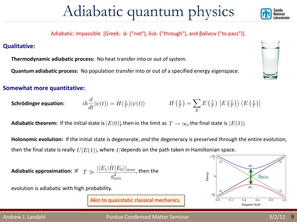
At the point of closest approach, the denominator $E_n-E_k$ is at its minimum, making the system most susceptible to non-adiabatic transitions.

3. Breakdown: Landau-Zener Transitions

Let's study a canonical model where this breakdown can be solved exactly: the Landau-Zener problem. This describes a two-level system whose energy levels would cross, but are pushed apart by a constant interaction. This is the canonical model for an avoided crossing.

The Landau-Zener analysis gives us a beautiful, physical picture of the adiabatic condition. The system has two characteristic timescales:

1. Internal Timescale: The time it takes for the system to oscillate between the two states at the point of minimum separation. This is related to the Rabi period, $T_{Rabi}\sim \hslash /|H_{12}|$, where $2|H_{12}|$ is the minimum energy gap.
2. External Timescale: The time the system spends in the "interaction region" where the levels are close. This is related to the rate of change of the Hamiltonian, ${\tau }_D\sim |H_{12}|/|\alpha |$, where $\alpha$ is the speed at which the unperturbed levels cross.

The process is adiabatic if the system has enough time to oscillate many times while passing through the interaction region, i.e., ${\tau }_D\gg T_{Rabi}$. If the change is too fast, the system doesn't have time to "adjust" and may jump across the gap.

The probability of making such a non-adiabatic transition is given by the Landau-Zener formula:
$P_{LZ}=\exp \left(-2\pi \frac{|H_{12}{|}^2}{\hslash |\alpha |}\right)$
This formula beautifully quantifies our intuition: a larger gap ($|H_{12}|$) or a slower crossing speed ($|\alpha |$) leads to an exponentially suppressed probability of jumping to the other state.

4. Application: The Born-Oppenheimer Approximation

The adiabatic theorem is the theoretical foundation for one of the most important approximations in quantum chemistry and condensed matter physics: the Born-Oppenheimer approximation. Your background in both physics and chemistry makes this a particularly relevant example.

The core idea is a separation of timescales:

• Electrons are light ($m_e$) and move very fast.
• Nuclei are thousands of times heavier ($M_N$) and move very slowly.

From the perspective of the fast-moving electrons, the positions of the nuclei $\{\vec{R}\}$ are slowly changing parameters in their Hamiltonian, $H_{elec}(\{\vec{R}\})$. According to the adiabatic theorem, if the electronic system starts in its ground state, it will remain in the ground state corresponding to the instantaneous positions of the nuclei.

This allows us to first solve the electronic problem for a fixed nuclear configuration to find the electronic ground state energy, $E_{elec}(\{\vec{R}\})$. This energy then acts as an effective potential energy surface for the much slower motion of the nuclei. This approximation is what allows us to talk about molecular shapes and potential energy surfaces, and it is fundamental to calculating properties like phonon modes in crystals.

Conclusion

Today we have explored the limit of slowly-varying Hamiltonians, a stark contrast to the rapidly oscillating perturbations of our last lesson.

Key Takeaways:

• The Adiabatic Theorem states that if a system starts in an eigenstate of a slowly-varying Hamiltonian, it will remain in the corresponding instantaneous eigenstate, provided the energy levels are non-degenerate.
• During this evolution, the wavefunction acquires both a dynamical phase, related to the integrated energy, and a geometric (Berry) phase, which depends only on the path taken in parameter space.
• The condition for adiabaticity is that the timescale of the Hamiltonian's change must be much longer than the system's internal timescales, which are set by the inverse of the energy gaps. This condition is hardest to meet at an avoided crossing.
• Landau-Zener theory provides an exact solution for the probability of non-adiabatic transitions at an avoided crossing, showing it's exponentially suppressed with the square of the energy gap and the slowness of the process.
• The Born-Oppenheimer approximation, a cornerstone of chemical and condensed matter physics, is a direct and powerful application of the adiabatic theorem.

Preview of the next lesson:
We have now studied two extremes: fast, oscillatory perturbations and very slow, gradual changes. What about the third case: a very sudden, near-instantaneous change in the Hamiltonian? This is the realm of the sudden approximation. In our next lesson, we will see how to calculate the system's state after such an abrupt change, completing our trifecta of fundamental time-dependent approximation methods.