Autoregressive Language Modeling: GPT's Core

Hello! Welcome to the sixth lesson in our module on LLM and Transformer Fundamentals.

In our last lesson, we assembled a complete Transformer decoder block, understanding the roles of masked self-attention, feed-forward networks, layer normalization, and residual connections. We now have the fundamental building block of models like GPT.

This lesson focuses on how we train this architecture to become a powerful language model. Our learning outcome is to describe the process of autoregressive language modeling (next-token prediction) and its role in GPT-style pretraining. We'll explore the simple yet profound objective that allows these models to learn from vast amounts of text and then use that knowledge to generate coherent new text.

Understanding this training-to-inference pipeline is critical. The design of the pretraining task directly dictates how inference must be performed, a distinction that is crucial in production systems like the Bedrock infrastructure you work with.

1. The Core Idea: Next-Token Prediction

At its heart, a GPT-style language model is a highly sophisticated next-token predictor. The core objective is simple: given a sequence of tokens, predict the very next token. This process is often called autoregressive language modeling.

"Autoregressive" means that the model's predictions depend on its own previous outputs. During generation, the token it predicts at step t becomes part of the input for predicting the token at step t+1.

Let's start with a high-level overview from Jay Alammar's excellent "The Illustrated GPT-2" post.

The key insight here is that this simple objective can be applied to any text without needing human-created labels. This is known as self-supervised learning. The text itself provides the supervision: the next token in the sequence is the "label" for the preceding tokens. This is what allows us to pretrain models on massive, web-scale datasets.

2. The Pretraining Process: Learning from Data

During pretraining, the goal is to teach the model the statistical patterns of language. Given your work on high-throughput systems, the efficiency of this process is particularly interesting. The model learns to predict the next token for every position in a sequence simultaneously in a single forward pass.

2.1. Preparing the Data

First, we need to transform raw text into a format the model can use: batches of input and target tensors. A single sequence of text provides multiple training examples.

For a sequence [t1, t2, t3, t4]:

• When the input is [t1], the target is t2.
• When the input is [t1, t2], the target is t3.
• When the input is [t1, t2, t3], the target is t4.

Andrej Karpathy's "Let's build GPT" video provides a fantastic, practical demonstration of how to prepare data for training.

2.2. The Training Forward Pass

Once we have a batch of inputs (x) and targets (y), a training step proceeds as follows:

1. Get Embeddings: The input token IDs are converted into token and positional embeddings.
2. Process through Decoder Blocks: The resulting vectors are passed through the stack of Transformer decoder blocks we studied in the last lesson. The causal mask is critical here, ensuring that the prediction for position i only uses information from tokens 0 to i.
3. Get Logits: The output of the final decoder block is a sequence of vectors. Each vector is passed through a final linear layer (often called the "language model head") to produce a score vector (logits) the size of the vocabulary.
4. Calculate Loss: A softmax function is applied to the logits to create a probability distribution. The Cross-Entropy Loss is then calculated between this predicted distribution and the one-hot encoded ground truth target token.
5. Aggregate and Backpropagate: The loss is averaged across all positions in the sequence and all sequences in the batch. This final loss value is then used to update all the model's parameters via backpropagation.

This article provides a very clear text-based walkthrough of this process.

3. The Inference Process: Autoregressive Generation

While training is parallel, inference (generating new text) is a strictly sequential, one-token-at-a-time process. This is the autoregressive nature of the model in action.

The process works like a loop:

1. Start with an initial sequence (the prompt).
2. Pass the sequence through the model.
3. Take the output vector corresponding to the very last token only.
4. Convert this vector into a probability distribution over the vocabulary.
5. Sample a new token from this distribution.
6. Append the new token to the sequence.
7. Repeat from step 2.

This animation perfectly illustrates the process:

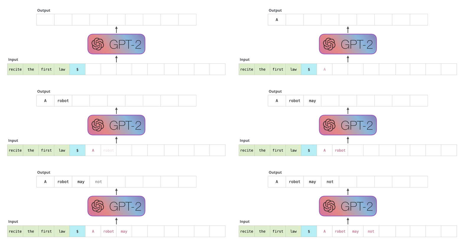
To solidify this concept, let's watch Karpathy implement a simple generate function. Even though he's using a simpler bigram model at this stage, the autoregressive logic is identical to what a full GPT model uses.

4. Training vs. Inference: A Tale of Two Modes

It's vital to distinguish between the parallel efficiency of training and the serial nature of inference. Your work on Rudi, scheduling inference requests, deals directly with the challenges of this serial generation process.

• During Training: We feed the model the entire sequence at once and compute the loss for all next-token predictions in parallel. This is possible because the causal mask prevents any position from seeing future tokens.
• During Inference: We don't have the future tokens. We must generate them one by one, feeding the model's own output back to it in a loop.

This video from CodeEmporium provides an exceptionally clear explanation of this crucial difference.

Conclusion

In this lesson, we've demystified the process that powers GPT-style models. We've seen how a simple, self-supervised objective—next-token prediction—when combined with the Transformer decoder architecture and massive datasets, creates a powerful generative model.

Key Takeaways:

• Autoregressive Language Modeling: The core task is predicting the next token in a sequence based on the preceding ones.
• Self-Supervised Pretraining: Models are trained on vast amounts of unlabeled text, where the text itself provides the input sequences and the target next tokens.
• Training is Parallel: During pretraining, the model predicts the next token for all positions in a sequence simultaneously in a single forward pass, enabled by the causal attention mask.
• Inference is Serial: During generation, the model produces text one token at a time, feeding its own output back as input for the next step in a loop.
• The Causal Mask is Key: This architectural feature makes the efficient, parallel training process a valid proxy for the slow, serial inference process.

Next Lesson Preview

We've learned that during inference, the model produces a probability distribution over the entire vocabulary for the next token. But how do we choose a token from that distribution? Simply picking the most likely one isn't always best. In our next lesson, we will compare common decoding strategies (greedy, beam search, top-k/top-p sampling) and the effect of temperature, exploring the trade-offs between creativity, coherence, and correctness in generated text.