Elementary Symmetric Polynomials and Characteristic Polynomials

Recommended resources

The freely available resources this lesson will direct you to.

Hello! Welcome to the fourth lesson in our course.

Introduction

In our previous work, we've been setting up the core optimization problem from the paper. We've seen how to represent solutions to linear difference equations and how the behavior is governed by the roots of the characteristic polynomial.

Today, we shift our focus to the algebraic machinery the paper uses to solve this problem. The abstract mentions "symmetric functions" and "Schur positivity." To understand these, we first need to build a foundation.

This lesson corresponds to the first learning outcome in Module 4: Define elementary symmetric polynomials and relate them to the coefficients of a characteristic polynomial. We will explore what makes a polynomial "symmetric" and then define a special class of them—the elementary symmetric polynomials. The key insight will be seeing how these polynomials provide a direct bridge between the roots of a polynomial (like our characteristic roots) and its coefficients.

This is a crucial step. The paper's proof strategy involves manipulating the characteristic roots to find an optimal configuration. Understanding the relationship between roots and coefficients via symmetric polynomials is the first step in appreciating that strategy.

1. What is a Symmetric Polynomial?

Before we dive into the "elementary" ones, let's start with the broader concept. A symmetric polynomial is a multivariate polynomial that remains unchanged if you swap any of its variables.

For example, consider the polynomial in three variables $X_{1}, X_{2}, X_{3}$ :
$P (X_{1}, X_{2}, X_{3}) = X_{1}^{2} + X_{2}^{2} + X_{3}^{2} + X_{1} X_{2} X_{3}$
If you swap $X_{1}$ and $X_{2}$ , you get:
$P (X_{2}, X_{1}, X_{3}) = X_{2}^{2} + X_{1}^{2} + X_{3}^{2} + X_{2} X_{1} X_{3}$
This is identical to the original polynomial. The same holds for any other permutation of the variables. This invariance is the defining feature of a symmetric polynomial.

Symmetric polynomials are fundamental in algebra because they naturally describe properties of a set of objects (like the roots of a polynomial) that don't depend on the order of those objects.

To get a more formal perspective, please read the short introductory section of the following resource.

Symmetric polynomial

This Wikipedia article on Symmetric polynomials provides a concise formal definition and explains why they are so relevant to studying the roots of a polynomial.

Please read the first three paragraphs of the article, down to the sentence ending with '...as a polynomial expression in the coefficients of the polynomial.' Focus on the formal definition involving permutations.

2. Elementary Symmetric Polynomials

Among all symmetric polynomials, there is a special set that acts as the fundamental building blocks: the elementary symmetric polynomials. Any other symmetric polynomial can be constructed from them.

For a set of $n$ variables ${X_{1}, X_{2}, \dots, X_{n}}$ , the $k$ -th elementary symmetric polynomial, denoted $e_{k} (X_{1}, \dots, X_{n})$ , is the sum of all distinct products of $k$ of these variables.

Let's make this concrete for $n = 4$ variables ${X_{1}, X_{2}, X_{3}, X_{4}}$ :

$e_{1}$ : Sum of all single variables.
$e_{1} (X_{1}, X_{2}, X_{3}, X_{4}) = X_{1} + X_{2} + X_{3} + X_{4}$
$e_{2}$ : Sum of all products of two distinct variables.
$e_{2} (X_{1}, X_{2}, X_{3}, X_{4}) = X_{1} X_{2} + X_{1} X_{3} + X_{1} X_{4} + X_{2} X_{3} + X_{2} X_{4} + X_{3} X_{4}$
$e_{3}$ : Sum of all products of three distinct variables.
$e_{3} (X_{1}, X_{2}, X_{3}, X_{4}) = X_{1} X_{2} X_{3} + X_{1} X_{2} X_{4} + X_{1} X_{3} X_{4} + X_{2} X_{3} X_{4}$
$e_{4}$ : The product of all four variables.
$e_{4} (X_{1}, X_{2}, X_{3}, X_{4}) = X_{1} X_{2} X_{3} X_{4}$

By convention, $e_{0} = 1$ (the empty product), and for $k > n$ , $e_{k} = 0$ since you can't choose $k$ distinct variables from a set of $n$ .

To solidify this definition, please review the following resource.

Elementary symmetric polynomial

The Wikipedia article on Elementary symmetric polynomials offers a clear, formal definition and several helpful examples.

Please read the 'Definition' and 'Examples' sections. Pay attention to the general formula using summation over index subsets.

3. The Connection to Polynomial Coefficients: Vieta's Formulas

Now we arrive at the central point of this lesson. Why are these polynomials so important for our problem? Because they provide a direct link between the roots of a polynomial and its coefficients.

Let's start with a simple monic quadratic polynomial with roots $z_{1}$ and $z_{2}$ :
$P (z) = (z - z_{1}) (z - z_{2}) = z^{2} - (z_{1} + z_{2}) z + z_{1} z_{2}$
Notice the coefficients:

The coefficient of $z^{1}$ is $- (z_{1} + z_{2}) = - e_{1} (z_{1}, z_{2})$ .
The constant term (coefficient of $z^{0}$ ) is $z_{1} z_{2} = e_{2} (z_{1}, z_{2})$ .

This pattern generalizes. For a monic polynomial of degree $n$ with roots $z_{1}, \dots, z_{n}$ ,
$P (z) = \prod_{i = 1}^{n} (z - z_{i}) = z^{n} - e_{1} (z) z^{n - 1} + e_{2} (z) z^{n - 2} - \dots + (- 1)^{n} e_{n} (z)$
where $z = (z_{1}, \dots, z_{n})$ .

This set of relations is known as Vieta's formulas.

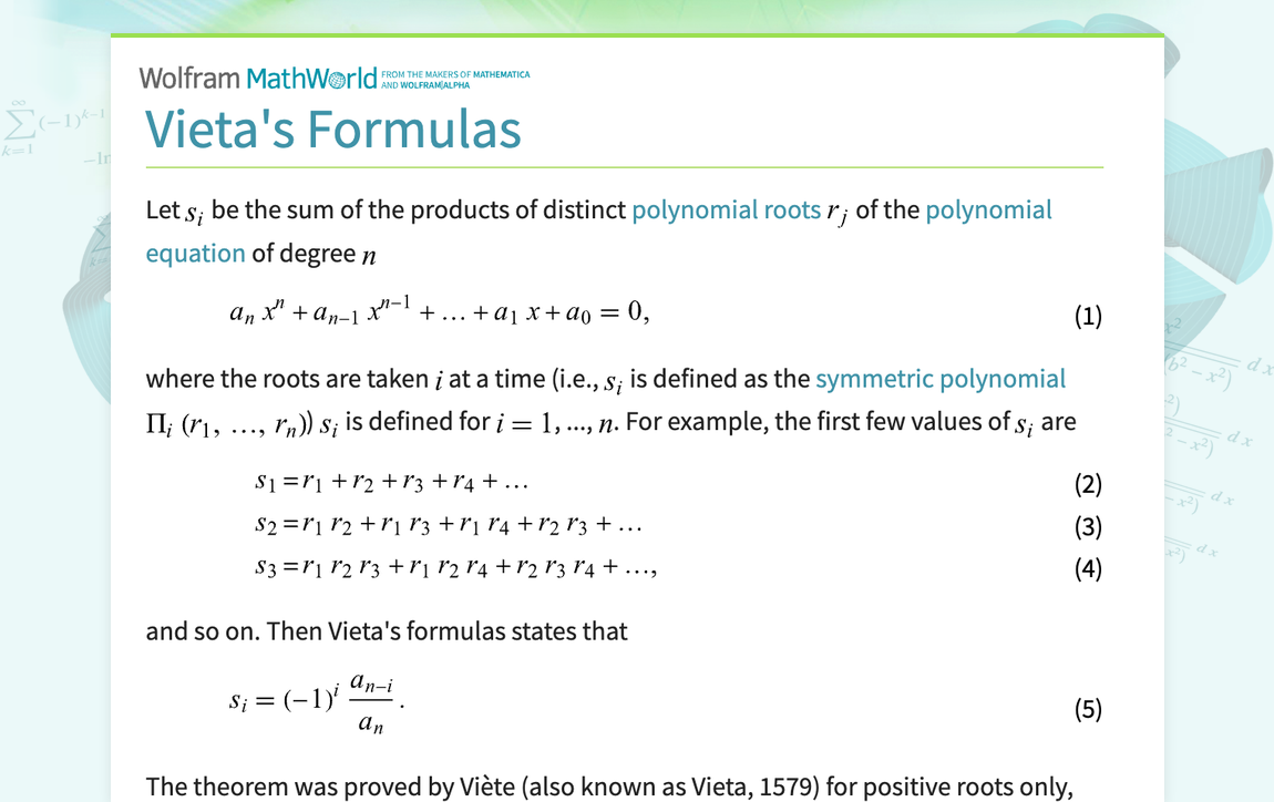
The next reading confirms this relationship and connects it directly to the characteristic polynomial of a matrix, which should be a familiar concept from your physics background.

Elementary symmetric polynomial

This section from the 'Elementary symmetric polynomial' article formalizes the connection we just discussed.

Please read the 'Properties' section. Focus on the identity that expands the product of linear factors and the subsequent application to the characteristic polynomial of a matrix. Note the connection to trace and determinant.

4. Application to Our Problem

In the context of our course, we are concerned with the characteristic polynomial of a linear difference equation. The roots of this polynomial, $λ_{1}, \dots, λ_{n}$ , are the "characteristic roots" mentioned in the paper's abstract.

Let the characteristic polynomial be:
$P (z) = z^{n} + c_{n - 1} z^{n - 1} + \dots + c_{1} z + c_{0}$
From Vieta's formulas, we know that these coefficients $c_{k}$ are determined by the elementary symmetric polynomials of the roots $λ_{i}$ :

$c_{n - 1} = - e_{1} (λ_{1}, \dots, λ_{n})$
$c_{n - 2} = e_{2} (λ_{1}, \dots, λ_{n})$
...
$c_{0} = (- 1)^{n} e_{n} (λ_{1}, \dots, λ_{n})$

This is a powerful link. It means that the coefficients of the difference equation are symmetric functions of its characteristic roots. Given your background, you'll recognize that $e_{1} (λ)$ is the trace of the system's companion matrix, and $e_{n} (λ)$ is its determinant (up to a sign).

The image below, from a lecture on this topic, provides an excellent visualization of this exact relationship.

This image illustrates the direct relationship between the coefficients of a characteristic polynomial $P_A(t)$ and the elementary symmetric polynomials ($S_k$ in this notation) of the matrix A's eigenvalues $\lambda_1, \dots, \lambda_n$.

This connection is the foundation for the paper's algebraic approach. The problem is to choose the roots $λ_{i}$ within a certain disk to maximize the solution's amplitude. By expressing parts of the problem in terms of symmetric polynomials, the authors can leverage powerful theorems from algebra to find the optimal configuration of these roots.

Conclusion

In this lesson, we have introduced a key component of the algebraic toolkit needed to understand the paper.

Key Takeaways:

Symmetric polynomials are invariant under the permutation of their variables.
Elementary symmetric polynomials ( $e_{k}$ ) are the basic building blocks, formed by summing all products of $k$ distinct variables.
Vieta's formulas establish a direct relationship between the coefficients of a monic polynomial and the elementary symmetric polynomials of its roots.
This allows us to express the coefficients of a characteristic polynomial in terms of symmetric functions of its characteristic roots (eigenvalues).

This final point is what we will carry forward. The problem of choosing optimal roots can be viewed through the lens of their symmetric combinations.

Preview of the Next Lesson:
We will continue building our algebraic toolkit by introducing Schur polynomials. These form another, more complex basis for the space of symmetric functions. We will then discuss the concept of Schur positivity, which is the linchpin of the main proof in the paper.