Solving Systems with Matrix Methods

Recommended resources

The freely available resources this lesson will direct you to.

Hello! Welcome to the sixth lesson in our foundational module on linear algebra.

In our last lesson, we established a crucial connection: any linear transformation can be represented by a matrix. We concluded by framing the equation $A x = b$ in this new light: we are searching for an input vector $x$ that, when transformed by the linear map represented by matrix $A$ , lands on the output vector $b$ .

Today, we will learn a systematic method to find that input vector $x$ . Our learning outcome is to solve systems of linear equations using matrix methods, specifically Gaussian elimination. We will explore both the step-by-step procedure of this powerful algorithm and, crucially, the formal mathematical proof that guarantees its validity.

1. From Equations to Matrices

A system of $m$ linear equations in $n$ unknowns can be a bit unwieldy. Our first step is to encode all the necessary information into a compact matrix structure.

A system like:

a_{11} x_{1} + a_{12} x_{2} + \dots + a_{1 n} x_{n} a_{21} x_{1} + a_{22} x_{2} + \dots + a_{2 n} x_{n} ⋮ a_{m 1} x_{1} + a_{m 2} x_{2} + \dots + a_{mn} x_{n} = b_{1} = b_{2} ⋮ = b_{m}

is equivalent to the matrix equation $A x = b$ . For computational purposes, we combine the coefficient matrix $A$ and the right-hand side vector $b$ into a single matrix called the augmented matrix, denoted $[A ∣ b]$ .

Systems of Linear Equations

To formalize this setup, please read this brief excerpt from a linear algebra textbook by Cheney and Kincaid. It introduces the standard notation for systems of linear equations and defines the coefficient matrix, vector of unknowns, and the augmented matrix.

Read the section 'General Systems of Linear Equations' (starts on page 6). Focus on the definitions of the four arrays: the coefficient matrix A, the vector of unknowns x, the right-hand-side vector b, and the augmented matrix [A | b].

The augmented matrix $[A ∣ b]$ contains all the numerical information of the system. We can now operate on the rows of this matrix to simplify the system without having to rewrite the variables $x_{1}, x_{2}, \dots$ at every step.

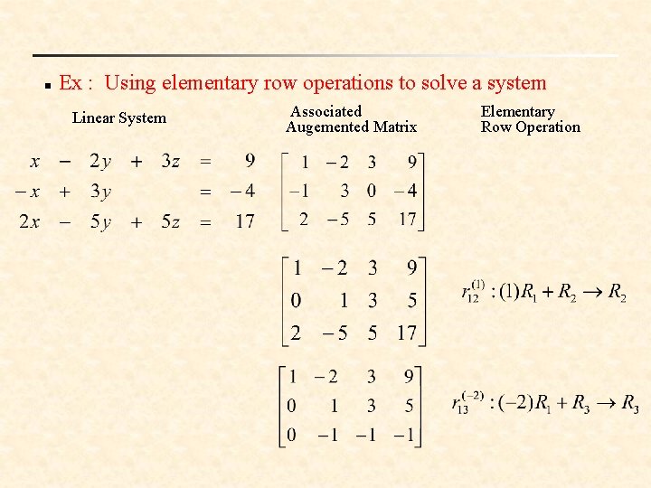
Elementary Row Operations for Solving Linear Systems — This image illustrates the process: a system of equations (left) is converted into its augmented matrix form (top right). Elementary row operations are then applied to this matrix to begin the solution process.

2. The Gaussian Elimination Algorithm

Gaussian elimination is a systematic procedure for transforming any augmented matrix into a simpler form from which the solution can be easily read. The goal is to produce an upper-triangular structure. This simpler form is called row echelon form.

The algorithm relies on three types of elementary row operations:

Replacement: Add a multiple of one row to another row.
Swap: Interchange two rows.
Scaling: Multiply a row by a non-zero scalar.

The following video provides a clear, step-by-step demonstration of the entire process.

Gaussian elimination | Lecture 10 | Matrix Algebra for Engineers

In this lecture, Jeffrey Chasnov walks through a complete example of Gaussian elimination. He demonstrates how to use the elementary row operations to reach an upper-triangular form and then how to use back substitution to find the solution.

Watch the video from 00:40 to 12:35. Pay attention to the three phases: Forming the augmented matrix (00:40 - 03:35). Applying row operations to create zeros below the main diagonal, reaching 'upper triangular form' (03:35 - 08:35). This is the 'forward elimination' phase. Solving the simplified system using 'back substitution' (08:35 - 12:35).

The Two Main Phases:

Forward Elimination: Using elementary row operations, we introduce zeros below the first non-zero entry in each row. These leading non-zero entries are called pivots. The result is a matrix in row echelon form, which has a staircase-like pattern of non-zero entries.
Back Substitution: Once the matrix is in row echelon form, the system is easy to solve. The last equation gives the value of one variable. Substituting this value into the second-to-last equation allows you to solve for another variable, and so on, working your way back up.

An extension of this method, often called Gauss-Jordan elimination, continues the process to create zeros above the pivots as well, and scales all pivots to be 1. The resulting reduced row-echelon form (RREF) makes the solution even more explicit, as it often results in an identity matrix on the left side, with the solution vector appearing on the right.

3. The Theory: Why Does Gaussian Elimination Work?

This is the most important question for our purposes. How can we be certain that these row operations—swapping equations, adding them together—don't change the set of solutions? The answer lies in a beautiful connection to the concepts from our previous lessons.

The core idea is that each elementary row operation is equivalent to left-multiplying the matrix by an invertible matrix, known as an elementary matrix.

To delve into the proof, we will first watch a video that outlines the argument, and then study the formal proof in a set of lecture notes.

Why Gaussian Elimination works

This video by Dr. Peyam directly addresses the question of why the method works. It presents the core argument that row reduction preserves the solution set because it's equivalent to multiplying by an invertible matrix.

Watch from 01:47 to 09:30. First, focus on the statement of the key fact: row reduction does not add or lose solutions. Then, follow the proof that demonstrates how the process of row reduction can be represented as multiplication by a single invertible matrix P.

Now, for the rigorous details. The following resource formally defines elementary matrices and proves their invertibility, solidifying the argument you just saw.

Gaussian elimination

These MIT lecture notes on Gaussian elimination provide the formal mathematical underpinnings you're looking for. The section on elementary row operations is particularly relevant.

Please read Section 3, 'Elementary row operations' (starts on page 6). Focus on: The formal definitions of the four types of elementary row operations (M, L, U, E). The corresponding elementary row matrices. Proposition 3.4, which formally proves that these matrices are invertible and, therefore, that elementary row operations do not change the solution set.

To summarize the proof:
Let an original system be $A x = b$ . Applying a sequence of row operations is equivalent to multiplying by a sequence of elementary matrices $E_{k}, \dots, E_{2}, E_{1}$ . Let $P = E_{k} \dots E_{2} E_{1}$ . The new system is $(P A) x = P b$ .

If $x_{0}$ is a solution to the original system, then $A x_{0} = b$ . Multiplying by $P$ gives $P (A x_{0}) = P b$ , so $(P A) x_{0} = P b$ . Thus, $x_{0}$ is also a solution to the new system.
Conversely, because each elementary matrix is invertible, their product $P$ is also invertible. If $x_{0}$ is a solution to the new system, then $(P A) x_{0} = P b$ . Multiplying by $P^{- 1}$ gives $P^{- 1} (P A) x_{0} = P^{- 1} P b$ , which simplifies to $A x_{0} = b$ . Thus, $x_{0}$ is a solution to the original system.

The two systems have identical solution sets. This proves that Gaussian elimination is a valid method for finding solutions.

4. Existence and Uniqueness of Solutions

The final reduced row-echelon form of the augmented matrix tells us everything about the nature of the solution.

No Solution (Inconsistent System): If the RREF contains a row of the form $[00 \dots 0 ∣ c]$ where $c$ is a non-zero number, the system is inconsistent. This row corresponds to the equation $0 = c$ , which is a contradiction. This is equivalent to saying the augmented matrix has a pivot in its final column.
At Least One Solution (Consistent System): If there is no such contradictory row, the system is consistent. We then have two sub-cases:
- Unique Solution: The system has a unique solution if every column in the coefficient part of the matrix (the part corresponding to $A$ ) is a pivot column. This means there are no free variables.
- Infinite Solutions: If there is at least one column in the coefficient part of the matrix that is not a pivot column, the corresponding variable is a free variable. We can assign it any value, and the other variables will be determined accordingly. This gives rise to an infinite set of solutions, which can be expressed parametrically.

Test your understanding!

After performing Gaussian elimination, you arrive at the following augmented matrix in reduced row-echelon form:

100010 - 2 30 ∣ ∣ ∣ 5 - 1 0

Write the general solution for the system $(x_{1}, x_{2}, x_{3})$ .

Show answer

First, let's translate the matrix back into equations:

$x_{1} - 2 x_{3} = 5$
$x_{2} + 3 x_{3} = - 1$
$0 = 0$

The third equation is trivial and tells us the system is consistent. The pivot columns are the first and second columns. The third column does not have a pivot, so $x_{3}$ is a free variable. We can set $x_{3} = t$ , where $t$ is any real number (a parameter).

Now, we express the pivot variables ( $x_{1}, x_{2}$ ) in terms of the free variable:

From the first equation: $x_{1} = 5 + 2 x_{3} = 5 + 2 t$
From the second equation: $x_{2} = - 1 - 3 x_{3} = - 1 - 3 t$

The general solution is the set of all vectors $x$ of the form:

x = x_{1} x_{2} x_{3} = 5 + 2 t - 1 - 3 t t

We can separate this into a particular solution and a homogeneous solution:

x = 5 - 1 0 + t 2 - 3 1

This represents a line in $R^{3}$ .

Conclusion

In this lesson, we moved from the abstract formulation of a linear system to a concrete, algorithmic solution method.

Key Takeaways:

A system of linear equations $A x = b$ can be solved by applying Gaussian elimination to the augmented matrix $[A ∣ b]$ .
The algorithm uses elementary row operations (replacement, swap, scale) to transform the matrix into row echelon form or reduced row-echelon form.
The procedure is guaranteed to work because elementary row operations are equivalent to multiplication by invertible elementary matrices, which preserves the solution set of the system.
The final form of the matrix reveals whether the system has a unique solution, infinite solutions (in the case of free variables), or no solution (in the case of a contradiction).

In our next lesson, we will formalize some of the concepts we observed today. The number of pivots in the row-echelon form of a matrix is an intrinsic and deeply important property called its rank. The number of free variables relates to the dimension of the null space, or the nullity. We will define these terms and prove the fundamental rank-nullity theorem, which connects them.