Dijkstra's Algorithm: Finding the Shortest Path

Hello! Welcome to the final lesson in our module on Graph Algorithms.

In our previous lessons, we built a strong foundation in graph traversal. We started with BFS and DFS, then made them robust enough to handle complexities like disconnected components and self-loops. These algorithms are perfect for answering questions about reachability or exploring an entire graph, but they treat all paths as equal.

Today, we address a more nuanced problem common in network routing, task scheduling, and logistics: finding the cheapest or fastest path, not just any path. This lesson directly targets the learning outcome: Solve a shortest path problem on a weighted graph using Dijkstra's algorithm.

Your work on Rudi at AWS involves scheduling and routing inference requests, where "cost" could mean latency, compute resources, or even token usage. Dijkstra's algorithm is the canonical tool for solving exactly this type of optimization problem, making it a crucial addition to your software engineering toolkit.

1. From Unweighted to Weighted Shortest Path

In an unweighted graph, the shortest path is the one with the fewest edges. Breadth-First Search (BFS) is guaranteed to find this because it explores the graph layer by layer.

However, in a weighted graph, each edge has a "cost" or "weight". The shortest path is the one where the sum of the weights of its edges is minimized.

Consider a path from A to B with 5 edges of weight 1 each (total weight 5). Another path might have only 2 edges, but with weights 3 and 4 (total weight 7). A simple BFS would incorrectly choose the 2-edge path. We need an algorithm that accounts for these weights.

This is where Dijkstra's algorithm comes in. It's a greedy algorithm that finds the single-source shortest path in a weighted graph, provided there are no negative edge weights.

2. The Core Idea: Greedy Selection and Relaxation

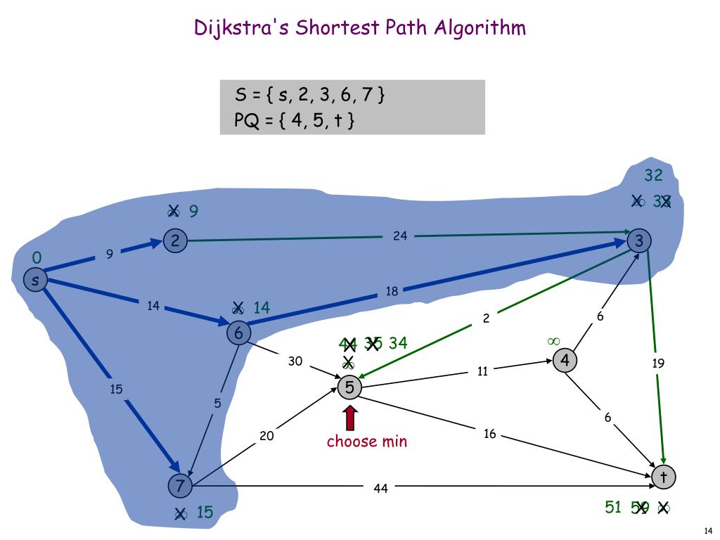
Dijkstra's algorithm works by iteratively building up a set of nodes for which the shortest path from the source is known.

At each step, it greedily selects the node that is "closest" to the source among all nodes not yet finalized. Once a node is selected, its path is considered final. Then, it updates the distances to its neighbors in a process called relaxation.

To get a solid grasp of this process, the following video provides an excellent conceptual breakdown.

As the video demonstrates, the algorithm maintains two key pieces of information:

1. A set of "visited" nodes whose shortest path from the source is finalized.
2. A data structure (e.g., an array or dictionary) storing the current shortest-known distance from the source to every other node. This is initialized to $\infty$ for all nodes except the source, which is 0.

The relaxation step for an edge from node u to node v is the core of the algorithm. It checks if the path to v through u is shorter than the currently known best path to v.

Mathematically, it's:

3. An Efficient Implementation with a Priority Queue

The naive approach shown in the first video involves scanning all unvisited nodes at each step to find the one with the minimum distance. For a graph with V vertices, this leads to an O(V^2) time complexity. We can do much better.

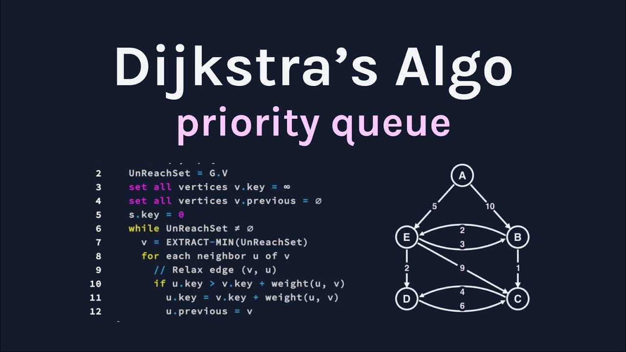
A more efficient implementation uses a priority queue (specifically, a min-heap) to store the unvisited nodes. The priority queue allows us to retrieve the node with the minimum distance in O(log V) time instead of O(V).

This video provides a detailed walkthrough of the priority queue-based approach, which is the standard and expected implementation in an interview setting.

Here is a summary of the algorithm using a priority queue:

1. Initialization:

   • Create a distances array, initialized to infinity for all nodes except the source (distances[source] = 0).
   • Create a min-priority queue and push the tuple (0, source).

2. Iteration:

   • While the priority queue is not empty:
     a. Pop the element with the smallest distance: (cost, position).
     b. If cost > distances[position], it means we've found a shorter path to this node already. continue.
     c. For each neighbor of position with edge weight w:
     i. If distances[position] + w < distances[neighbor]:
     - Update distances[neighbor] = distances[position] + w.
     - Push (distances[neighbor], neighbor) to the priority queue.

3. Completion:

   • Once the loop finishes, the distances array contains the shortest path distances from the source to all other nodes.

4. Production-Quality Implementation in Rust

Given your expertise, let's look at how to implement this idiomatically in Rust. The std::collections::BinaryHeap provides a max-heap by default. To use it as a min-heap for Dijkstra's, we need a clever wrapper struct that inverts the comparison logic.

The official Rust documentation for BinaryHeap actually uses Dijkstra's algorithm as its primary example. This is an excellent, authoritative resource for a production-quality implementation.

The Rust book you're following, Modern Data Structures and Algorithms in Rust, also provides a very similar implementation (resource_id: [LINK](https://dsar.rantai.dev/docs/part-iii/chapter-15/), section "Shortest Path Algorithms"). Seeing the same pattern in multiple high-quality sources confirms its importance.

The key takeaway from the Rust implementation is the pattern of creating a custom struct and implementing Ord and PartialOrd to tailor the behavior of a standard data structure like BinaryHeap to your specific algorithmic needs.

5. Complexity and Limitations

Time Complexity Trade-offs

• Naive (Array/List Scan): O(V^2). Simple to implement but slow on large graphs.
• Priority Queue (Binary Heap): O(E log V). The standard. Each vertex is popped once (V * log V), and each edge may result in a push (E * log V).

For sparse graphs, where the number of edges E is close to V, O(E log V) is a significant improvement over O(V^2). Your work on distributed systems likely involves graphs that are sparse rather than fully connected, making this efficient implementation critical.

The Critical Limitation: Negative Edge Weights

Dijkstra's greedy approach makes a crucial assumption: once we select a node and finalize its shortest path, we will never find an even shorter path to it later. This assumption holds true only if all edge weights are non-negative.

If a graph has a negative edge, the algorithm can produce incorrect results. If it has a negative-weight cycle, the algorithm can get stuck in an infinite loop.

For graphs with negative weights, other algorithms must be used, such as the Bellman-Ford algorithm (O(VE)) or, for Directed Acyclic Graphs, a linear-time algorithm based on topological sort.

Conclusion

You have now learned one of the most famous and useful algorithms in computer science. Dijkstra's algorithm elegantly solves the single-source shortest path problem for weighted graphs and serves as a building block for many more complex routing and optimization systems.

Key Takeaways:

• Dijkstra's algorithm finds the shortest path from a single source in a weighted graph using a greedy strategy.
• The core operation is relaxation, where the estimated distance to a node is updated if a shorter path is found.
• The efficient, standard implementation uses a min-priority queue to achieve a time complexity of O(E log V).
• In Rust, a BinaryHeap (a max-heap) can be turned into a min-heap by creating a wrapper struct and implementing a reversed Ord trait.
• The algorithm's critical limitation is that it does not work correctly with graphs that have negative edge weights.

Next Lesson Preview

With Dijkstra's, we've reached the end of our foundational graph algorithms module. We're now prepared to move into the next module, "Advanced Algorithmic Patterns." Our first lesson there will introduce dynamic programming, another powerful technique for solving optimization problems. While Dijkstra's greedily builds one path, dynamic programming systematically builds solutions to all smaller subproblems to find the overall optimum. This new paradigm will open up a whole new class of problems for you to solve.