Constrained Optimization with Lagrange Multipliers

Hello! Last lesson, you classified stationary points by examining the Hessian in every direction. A constraint changes which directions matter: a point can minimize a function among allowed positions even when its gradient is not zero. This lesson develops Lagrange multipliers to find those points, then shows how to decide which candidates are minima or maxima.

Extremes when movement is restricted

Suppose you want to optimize $f(x,y)$, but only at points satisfying

The equation $g=k$ describes the feasible curve. At a constrained extremum, moving a little along that curve cannot change $f$ to first order. Moving away from the curve is irrelevant, however steeply $f$ changes there.

The diagram shows the idea. The orange constraint line touches one of the blue level curves of $f$. A level curve that crosses the line would not generally mark an extremum: you could move along the line to reach values on either side of it.

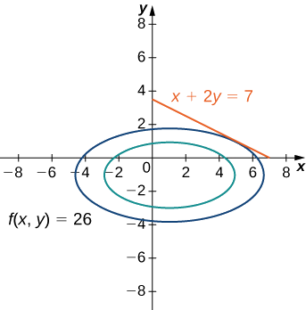
Watch the indicated parts of Lec 13: Lagrange multipliers from MIT OpenCourseWare. The lecturer uses a distance-to-the-origin problem to turn this picture into equations. Notice that the objective’s level curves and the constraint are different objects, even though both are drawn as curves in the same plane.

At a tangency, the two curves have the same tangent line. Gradients are perpendicular to their respective level curves, so the gradients must be parallel. We express that condition with a scalar $\lambda$, called a Lagrange multiplier:

In components, these are three equations for $x$, $y$, and $\lambda$:

Parallel includes the possibility that the gradients point in opposite directions, so $\lambda$ need not be positive. It can also be zero if $\nabla f=0$ at a feasible point.

Why the equation works

The geometric picture has a useful chain-rule interpretation. Parametrize a smooth portion of the constraint by $\mathbf{r}(t)=(x(t),y(t))$. Because every point on this path is feasible, $g(\mathbf{r}(t))=k$, and therefore

Thus the path’s tangent ${\mathbf{r}}^{\prime }(t)$ is perpendicular to $\nabla g$. At a local maximum or minimum of $f$ along the same path,

Both gradients are consequently perpendicular to the feasible tangent. In two dimensions, if $\nabla g\ne 0$, they must be scalar multiples. The same reasoning works on a smooth constraint surface in three dimensions: at an extremum, $\nabla f$ is perpendicular to every feasible tangent direction.

For another presentation of this argument, watch the later portion of the MIT lecture. The important phrase is unchanged to first order: $f$ need not remain constant as you walk along the constraint away from an extremum.

A compact way to organize the equations is to define the Lagrangian

Setting its three first partial derivatives to zero reproduces the two gradient equations and the constraint. This is an equation-generating device: making $\mathcal{L}$ stationary does not, by itself, prove that $f$ has a constrained minimum or maximum.

Solving a constrained minimum

Consider the quadratic energy-like function

subject to $x+2y=6$. Without the restriction, $E$ is smallest at $(0,0)$, but that point is infeasible. Put $g(x,y)=x+2y$. The multiplier equations are

The first two components give $2x=\lambda$ and $4y=2\lambda$, so $x=y=\lambda /2$. The constraint then gives $3x=6$, hence

We have found a candidate. Here we can prove it is the global constrained minimum by substituting $y=(6-x)/2$:

This check also shows why there is no maximum: the feasible line extends without bound, and the energy grows without bound along it. The multiplier equations locate stationary behavior on the constraint; they do not promise that both kinds of extremum exist.

The multiplier has one more interpretation when the constraint value varies. Replacing $6$ by $k$ gives the minimum $E_{\min }(k)=k^2/3$. Its derivative at $k=6$ is $4$, exactly the multiplier found above. With our sign convention $\mathcal{L}=f-\lambda (g-k)$, this sensitivity relation holds when the optimum varies smoothly:

Finding all candidates before comparing them

On a closed feasible curve, there may be several multiplier solutions. To see why keeping every algebraic branch matters, find the extrema of

With $g=x^2+y^2$, the equations are

Neither $x$ nor $y$ can be zero in a solution: if one were zero, the gradient equations would force the other to be zero, contradicting the constraint. Substituting one gradient equation into the other therefore gives $4{\lambda }^2=1$.

For $\lambda =1/2$, we have $y=x$, yielding $(1,1)$ and $(-1,-1)$, both with $f=1$. For $\lambda =-1/2$, we have $y=-x$, yielding $(1,-1)$ and $(-1,1)$, both with $f=-1$. Thus the constrained maximum is $1$ and the constrained minimum is $-1$.

Why is comparing these four values enough here? The feasible circle is closed and bounded, $f$ is continuous, and its constraint gradient $(2x,2y)$ never vanishes on the circle. Global extrema therefore exist and must appear among the multiplier candidates. On a noncompact constraint such as a line, existence needs a separate argument—as the preceding example showed.

Two constraints and the boundaries of the method

For a function of three variables restricted by two equations, a feasible tangent must respect both. At a regular constrained extremum, the objective gradient can be a combination of the two constraint gradients:

There is one multiplier per equality constraint. Read the selected passages from Gilbert Strang’s Calculus, Chapter 13, Section 13.7, for the Lagrangian formulation and the geometry of two constraints. Its worked three-dimensional example finds the closest point to the origin on the intersection of two planes.

For a short calculation with two constraints, minimize $f=x^2+y^2+z^2$ subject to $g=x+y+z=3$ and $h=x-y=0$. The equations become

The constraint $x=y$, together with the first two components, gives $\mu =0$. The remaining components then imply $x=y=z$; their sum is $3$, so the candidate is $(1,1,1)$, where $f=3$. It is a global minimum: for any feasible displacement $\mathbf{d}$ from $(1,1,1)$, the constraint requires $d_x+d_y+d_z=0$, and

Finally, remember what the multiplier equations assume. The usual one-constraint condition requires a regular feasible curve or surface, with $\nabla g\ne 0$ at the candidate. If that gradient vanishes, inspect the point separately; the parallel-gradient argument may fail. Likewise, if a problem restricts you to only part of a curve, check its endpoints as well. These are reasons to treat the equations as a systematic way to find candidates, not as a substitute for checking the feasible set.

Looking ahead

For an equality-constrained extremum, write down the objective and every constraint, solve the gradient equations together with those constraints, and then evaluate and justify the resulting candidates. The central change from last lesson is that first-order change must vanish only in feasible directions; the ordinary unconstrained Hessian test does not settle what happens along a constraint.

Next, you will turn from restricting variables to changing them in double and triple integrals, where the Jacobian determinant accounts for how a coordinate transformation scales area and volume.