Second-Order Multivariable Taylor Approximation

Recommended resources

The freely available resources this lesson will direct you to.

Hello! Last lesson, you used the gradient to find a field’s change per unit distance in a chosen direction. That is first-order information: it tells you the initial slope, but not how that slope changes as you move. Today you will add second derivatives to construct a second-order Taylor approximation near a specified point.

This local quadratic model is useful throughout higher physics. For example, near a reference configuration, it can describe how a potential changes with small displacements. The aim here is to build the model reliably; the next lesson will use its second-derivative matrix to analyze stationary points.

From a tangent plane to a curved local model

Let $f (x, y)$ be a smooth scalar field, and choose a reference point $(a, b)$ . Write a nearby point as $(a + h, b + k)$ , where $h$ and $k$ are displacements from the reference point. The first-order approximation is the tangent plane:

f (a + h, b + k) \approx f (a, b) + f_{x} (a, b) h + f_{y} (a, b) k .

This matches the value and both coordinate slopes of $f$ at $(a, b)$ . It cannot, however, bend as $f$ bends. A second-order approximation adds all the possible quadratic displacement terms: $h^{2}$ , $hk$ , and $k^{2}$ .

Watch the selected portion of M4ML - Multivariate Calculus - 4.8 Multivariate Taylor from Digital Media - Imperial College London. Its changing surfaces make the distinction between a tangent plane and a quadratic approximation visible before we calculate one.

M4ML - Multivariate Calculus - 4.8 Multivariate Taylor

Watch how the constant, linear, and quadratic models fit a surface near a chosen point, then see how their formulas are assembled.

Watch the surfaces for the geometric picture. Continue with the quadratic formula, paying particular attention to the mixed term, and matrix notation, which connects the approximation to the Jacobian you have already used.

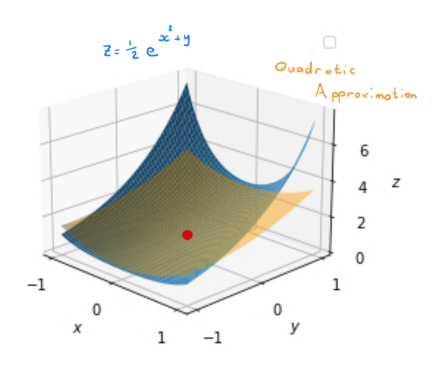
The image below shows why the reference point matters. The orange quadratic surface follows the blue function near the marked point, but a Taylor approximation is not intended to reproduce the entire surface.

The blue surface represents a nonlinear function, while the orange surface is a quadratic approximation constructed at the red reference point. Their separation farther from that point illustrates the local nature of the approximation.

Where the three quadratic terms come from

Your earlier chain-rule calculations provide a direct way to derive the formula. Hold the displacement $(h, k)$ fixed and travel from the reference point along the straight line

g (t) = f (a + t h, b + t k) .

Here $g$ is a function of just one variable. At $t = 0$ , you are at $(a, b)$ ; at $t = 1$ , you are at $(a + h, b + k)$ . The ordinary one-variable Taylor formula gives

g (1) \approx g (0) + g^{'} (0) + \frac{1}{2} g^{''} (0) .

The chain rule supplies the first derivative:

g^{'} (t) = f_{x} (a + t h, b + t k) h + f_{y} (a + t h, b + t k) k .

Differentiate once more. The displacement components are constants, but each partial derivative of $f$ changes along the line:

g^{''} (t) = f_{xx} (a + t h, b + t k) h^{2} + (f_{x y} + f_{y x}) (a + t h, b + t k) hk + f_{yy} (a + t h, b + t k) k^{2} .

For a sufficiently smooth function, the mixed partials agree: $f_{x y} = f_{y x}$ . Evaluating at $t = 0$ therefore gives the second-order Taylor polynomial about $(a, b)$ :

P_{2} (a + h, b + k) = f (a, b) + f_{x} (a, b) h + f_{y} (a, b) k + \frac{1}{2} f_{xx} (a, b) h^{2} + f_{x y} (a, b) hk + \frac{1}{2} f_{yy} (a, b) k^{2} .

The mixed term has no visible factor of $1/2$ because two equal mixed-derivative contributions combine before the whole quadratic expression is divided by two. Its presence matters: changing $x$ and $y$ together can affect the field differently from changing either coordinate alone.

In the more familiar $(x, y)$ notation, substitute $h = x - a$ and $k = y - b$ . Keeping these displacements visible is often safer than immediately expanding everything into powers of $x$ and $y$ .

Constructing an approximation at a specified point

Consider

f (x, y) = x e^{y} + x^{2} y

and construct $P_{2}$ about $(1, 0)$ . First, calculate the value and first derivatives:

f (1, 0) = 1, f_{x} = e^{y} + 2 x y, f_{y} = x e^{y} + x^{2} .

At the reference point, $f_{x} (1, 0) = 1$ and $f_{y} (1, 0) = 2$ . Thus the linear part is $1 + (x - 1) + 2 y$ .

Next find the three distinct second partials:

f_{xx} = 2 y, f_{x y} = e^{y} + 2 x, f_{yy} = x e^{y} .

Their values at $(1, 0)$ are $0$ , $3$ , and $1$ , respectively. With $h = x - 1$ and $k = y$ , the result is

P_{2} (1 + h, k) = 1 + h + 2 k + 3 hk + \frac{1}{2} k^{2} .

Equivalently,

P_{2} (x, y) = 1 + (x - 1) + 2 y + 3 (x - 1) y + \frac{1}{2} y^{2} .

Notice that there is no $h^{2}$ term: its coefficient is zero at this reference point. Also notice the $3 hk$ term. Omitting it would discard the largest second-order contribution for some directions of displacement.

To see the approximation at work, move to $(1.1, - 0.1)$ , so $h = 0.1$ and $k = - 0.1$ . The tangent-plane estimate is $0.9$ , whereas the quadratic estimate is

P_{2} (1.1, - 0.1) = 1 + 0.1 - 0.2 - 0.03 + 0.005 = 0.875.

The actual function value is approximately $0.87432$ . Here the quadratic term makes a substantial improvement. That comparison illustrates the benefit of second-order information, not a promise that the quadratic model will always be closer at every distance.

A dependable construction follows the order used above: choose the reference point; compute $f$ , the first partials, and the second partials there; then insert the displacements. Evaluating derivatives at the nearby point instead would produce a different calculation, not the Taylor polynomial about the requested point.

The Hessian packages the curvature

The Hessian collects the second partial derivatives into a matrix:

H_{f} (a, b) = (f_{xx} (a, b) f_{y x} (a, b) f_{x y} (a, b) f_{yy} (a, b)) .

If $d = (h, k)^{T}$ , the entire approximation becomes

P_{2} ((a, b) + d) = f (a, b) + \nabla f (a, b) \cdot d + \frac{1}{2} d^{T} H_{f} (a, b) d .

The gradient supplies the tangent-plane term. The Hessian supplies the quadratic correction. For the worked example,

H_{f} (1, 0) = (0331) .

Multiplying out $\frac{1}{2} d^{T} H_{f} (1, 0) d$ recovers $3 hk + \frac{1}{2} k^{2}$ . This compact form also works for three or more variables: the displacement vector and Hessian simply acquire more entries.

Read Multivariable Taylor polynomial example from Math Insight for a second construction. It uses one function at two different reference points, making it especially useful for checking why a Taylor polynomial must be tied to where it is built.

Multivariable Taylor polynomial example - Math Insight

Read Math Insight’s worked Gaussian example to connect the derivative-by-derivative method with the gradient–Hessian formula.

In “Multivariable Taylor polynomial example,” begin with the displayed matrix formula immediately below “Solution,” then read the calculations. Continue through the final expression for the polynomial at (1,2), just above “Thread navigation.” Compare the simple polynomial at (0,0) with the shifted one at (1,2); focus on how the derivative values and the displacement factors both change.

There is also a useful directional reading of the matrix expression. For a unit direction $u$ , put $d = s u$ . The approximation along that line is

f (p + s u) \approx f (p) + s \nabla f (p) \cdot u + \frac{s ^{2}}{2} u^{T} H_{f} (p) u .

You already know the coefficient of $s$ : it is the directional derivative. The coefficient involving $s^{2}$ describes how the field bends along that direction near $p$ . If the gradient vanishes, as it does at the origin in the Math Insight example, the quadratic term becomes the first potentially informative change.

The approximation remains local. If $f$ has continuous second derivatives near $p$ , then as the displacement approaches zero, the difference between $f (p + d)$ and $P_{2} (p + d)$ becomes small compared with $∥ d ∥^{2}$ . That is the precise sense in which the quadratic model captures the function through second order; it does not claim equality away from the reference point.

Looking ahead

A second-order Taylor approximation matches a function’s value, first derivatives, and second derivatives at the chosen point. Its linear term comes from the gradient; its quadratic term comes from the Hessian. Remember to express every term using displacements from the specified point, and include the mixed term when it is nonzero.

Next, you will use this same Hessian information to classify nondegenerate stationary points—places where the gradient, and therefore the entire linear term, vanishes.