Weight Initialization for Stable Gradients

Recommended resources

The freely available resources this lesson will direct you to.

Introduction

In our last lesson, we investigated the mathematical roots of the vanishing and exploding gradient problems, tracing them to the recursive application of the chain rule in deep networks. You learned that the repeated multiplication of weight matrices and activation function derivatives can cause the gradient signal to either shrink or grow exponentially, hindering or completely halting the learning process. We established the problem; now, we must formulate a solution.

This lesson focuses on one of the most effective strategies for promoting stable training: principled weight initialization. Instead of leaving initial weights to pure chance, we can use statistical reasoning to set them in a way that actively counteracts gradient instability from the very first forward pass. We will explore the theoretical justification for two landmark initialization schemes, Xavier/Glorot initialization and He initialization. You will derive the logic behind them and understand why the choice of initializer is critically linked to the network's activation functions.

The Principle of Stable Signal Propagation

The core idea behind modern weight initialization is to ensure that the "signal"—whether it's the activations in the forward pass or the gradients in the backward pass—maintains a consistent magnitude as it propagates through the network. In statistical terms, we want the variance of a layer's outputs to be equal to the variance of its inputs.

Let $a^{(l - 1)}$ be the activations of layer $l - 1$ and $a^{(l)}$ be the activations of layer $l$ . Our goals are twofold:

Forward Pass Stability: The variance of the activations should remain constant as we move forward through the network.
$\forall l, Var (a^{(l)}) = Var (a^{(l - 1)})$
Backward Pass Stability: The variance of the gradients of the cost with respect to the layer activations should remain constant as we backpropagate.
$\forall l, Var (\frac{\partial C}{\partial a ^{(l)}}) = Var (\frac{\partial C}{\partial a ^{(l - 1)}})$

If we can satisfy these conditions at initialization, we ensure that the signal gain across each layer is approximately 1. This prevents the exponential growth or decay that leads to exploding or vanishing gradients, respectively. Our task is to find the variance of the weight distribution, $Var (W)$ , that makes this possible.

Xavier/Glorot Initialization

In their seminal 2010 paper, Xavier Glorot and Yoshua Bengio proposed an initialization scheme specifically designed for networks with symmetric, zero-centered activation functions like the hyperbolic tangent ( $tanh$ ).

The derivation relies on a few key assumptions:

Weights $W$ and inputs $x$ are drawn from distributions with zero mean ( $E [W] = 0$ , $E [x] = 0$ ).
Weights, inputs, and gradients are all independent and identically distributed (i.i.d.).
The activation function $f$ is linear in the neighborhood of 0, with a derivative of 1 at 0 (i.e., $f^{'} (0) = 1$ ). The $tanh$ function satisfies this.

Theoretical Derivation

Let's derive the required weight variance. A neuron's pre-activation $z^{(l)}$ at layer $l$ is given by the weighted sum of activations from the previous layer, $a^{(l - 1)}$ :

z^{(l)} = i = 1 \sum n_{in} W_{i} a_{i}^{(l - 1)}

where $n_{in}$ is the number of input neurons (the "fan-in").

The variance of this sum is:

Var (z^{(l)}) = Var (i = 1 \sum n_{in} W_{i} a_{i}^{(l - 1)})

Using the properties of variance and our i.i.d. and zero-mean assumptions, this simplifies neatly. For independent variables $X$ and $Y$ with zero mean, $Var (X Y) = Var (X) Var (Y)$ . Since the sum involves $n_{in}$ such terms, we get:

Var (z^{(l)}) = n_{in} \cdot Var (W) \cdot Var (a^{(l - 1)})

Because we assume the activation function is approximately linear near the origin ( $a^{(l)} \approx z^{(l)}$ ), we have $Var (a^{(l)}) \approx Var (z^{(l)})$ . Substituting this in, we get:

Var (a^{(l)}) \approx n_{in} \cdot Var (W) \cdot Var (a^{(l - 1)})

For our forward pass stability condition, $Var (a^{(l)}) = Var (a^{(l - 1)})$ , to hold, the other terms must equal 1:

n_{in} \cdot Var (W) = 1 ⟹ Var (W) = \frac{1}{n _{in}}

A similar derivation for the backward pass (considering the gradients flowing back) yields a slightly different condition based on the number of output neurons (the "fan-out", $n_{o u t}$ ):

n_{o u t} \cdot Var (W) = 1 ⟹ Var (W) = \frac{1}{n _{o u t}}

To satisfy both of these conflicting constraints, Glorot and Bengio proposed a compromise: use the average of the fan-in and fan-out.

Var (W) = \frac{2}{n _{in} + n _{o u t}}

This is the core result of Xavier/Glorot initialization.

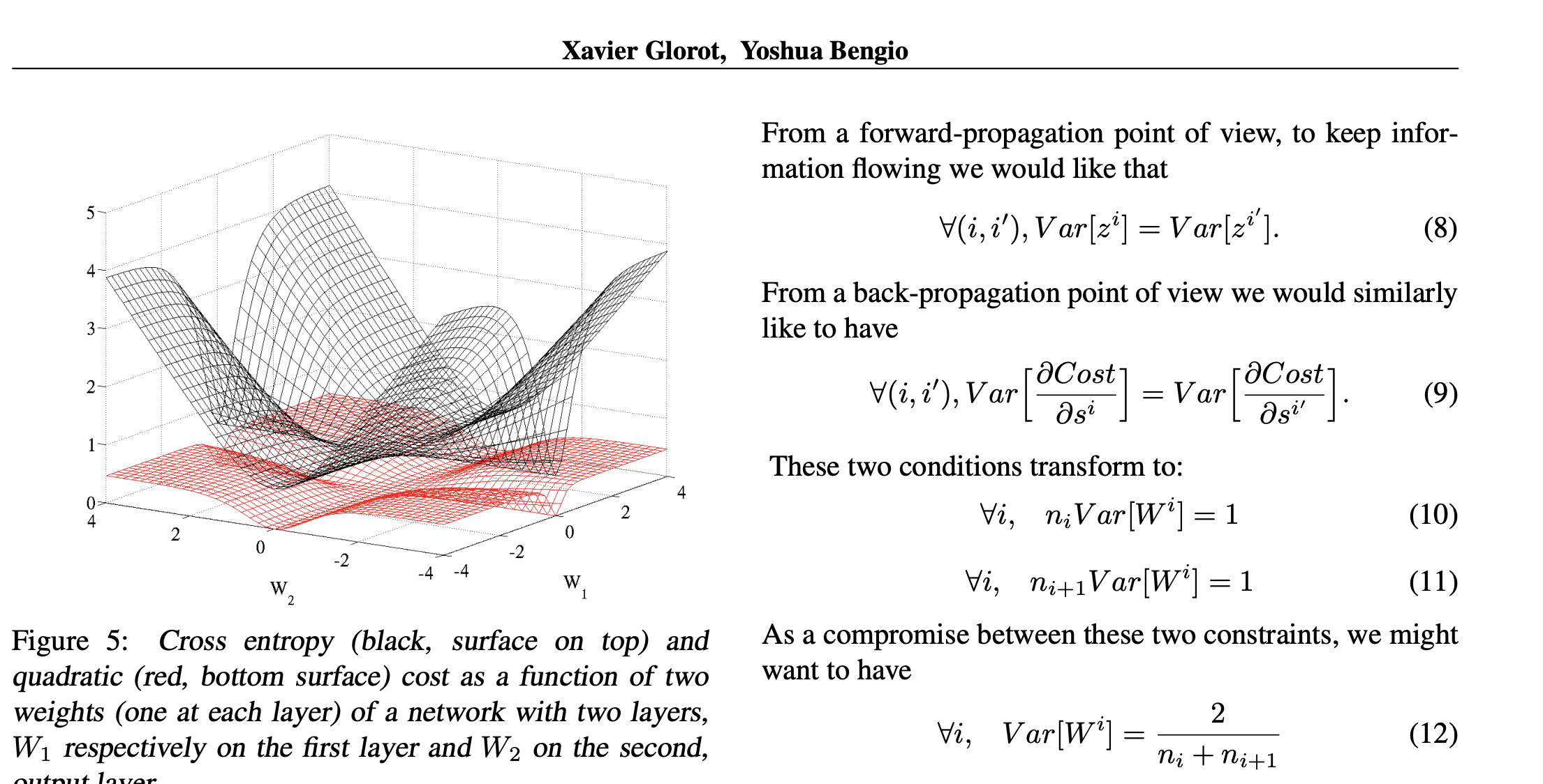
Figure from the original 2010 paper by Glorot and Bengio. To the right are the key equations showing the forward pass constraint (10), the backward pass constraint (11), and the final compromise (12) for the variance of the weights.

The following article provides a complete, step-by-step mathematical proof, which will be valuable for cementing your theoretical understanding.

Xavier Glorot Initialization in Neural Networks - Math Proof

This article from Towards Data Science meticulously derives the Xavier/Glorot initialization formula. It's an excellent resource for seeing all the mathematical steps laid out formally.

First, read the introduction and assumptions to ground yourself in the setup. Then, carefully follow the derivation for the forward pass, which arrives at the \text{Var}(W) = 1/n_{in} result. Next, work through the backward pass derivation to see how the \text{Var}(W) = 1/n_{out} condition arises. Finally, see how these are combined in the "Weight Distribution" section to arrive at the final formula.

Practical Implementation

Once we have the target variance, we can initialize the weights by drawing from a standard probability distribution with a mean of 0 and this specific variance.

Normal Distribution: We draw weights from $N (0, σ^{2})$ , where $σ^{2} = \frac{2}{n _{in} + n _{o u t}}$ .
Uniform Distribution: We draw weights from $U [- a, a]$ . The variance of this distribution is $\frac{a ^{2}}{3}$ . Setting this equal to our target variance gives $a = \frac{6}{n _{in} + n _{o u t}}$ .

The video below gives a great high-level overview and shows visualizations from the original paper, demonstrating the profound effect this initialization has on keeping gradients stable across layers.

L11.6 Xavier Glorot and Kaiming He Initialization

This video by Sebastian Raschka provides an intuitive explanation of Xavier/Glorot initialization and its effect on training dynamics.

First, watch the section covering the Xavier Glorot method. Focus on the core idea of scaling weights by a factor related to the fan-in. Then, pay close attention to the visualizations comparing a network with and without this initialization. Notice how the gradients in the bottom plot remain in a healthy range across all layers, solving the vanishing gradient problem seen in the top plot.

He Initialization

Xavier initialization works well for symmetric activations like tanh, but what about the Rectified Linear Unit (ReLU), the most common activation in modern networks? ReLU is defined as $f (x) = max (0, x)$ . It is not zero-centered, and its derivative is not 1 at the origin (it's undefined, but taken as 0 or 1 by convention). These violations of the Xavier assumptions mean we need a different approach.

In 2015, Kaiming He and his colleagues proposed an initialization scheme tailored for ReLU. The key insight is that because ReLU sets all negative inputs to zero, it effectively "kills" half of the input distribution. This cuts the variance of the signal in half at each layer.

Theoretical Derivation

To compensate for this halving of variance, we need to adjust our weight initialization. The derivation follows a similar path to Xavier's, but it accounts for the properties of ReLU. The forward pass variance equation becomes:

Var (z^{(l)}) = \frac{1}{2} n_{in} \cdot Var (W) \cdot Var (z^{(l - 1)})

The extra $\frac{1}{2}$ factor comes from the fact that $E [(a^{(l - 1)})^{2}] = \frac{1}{2} Var (z^{(l - 1)})$ for an input $z$ passed through a ReLU.

Now, for our stability condition $Var (z^{(l)}) = Var (z^{(l - 1)})$ to hold, we need:

\frac{1}{2} n_{in} \cdot Var (W) = 1 ⟹ Var (W) = \frac{2}{n _{in}}

Interestingly, the derivation for the backward pass also leads to the same result. There is no need for a compromise. The He initialization is simply defined by the fan-in.

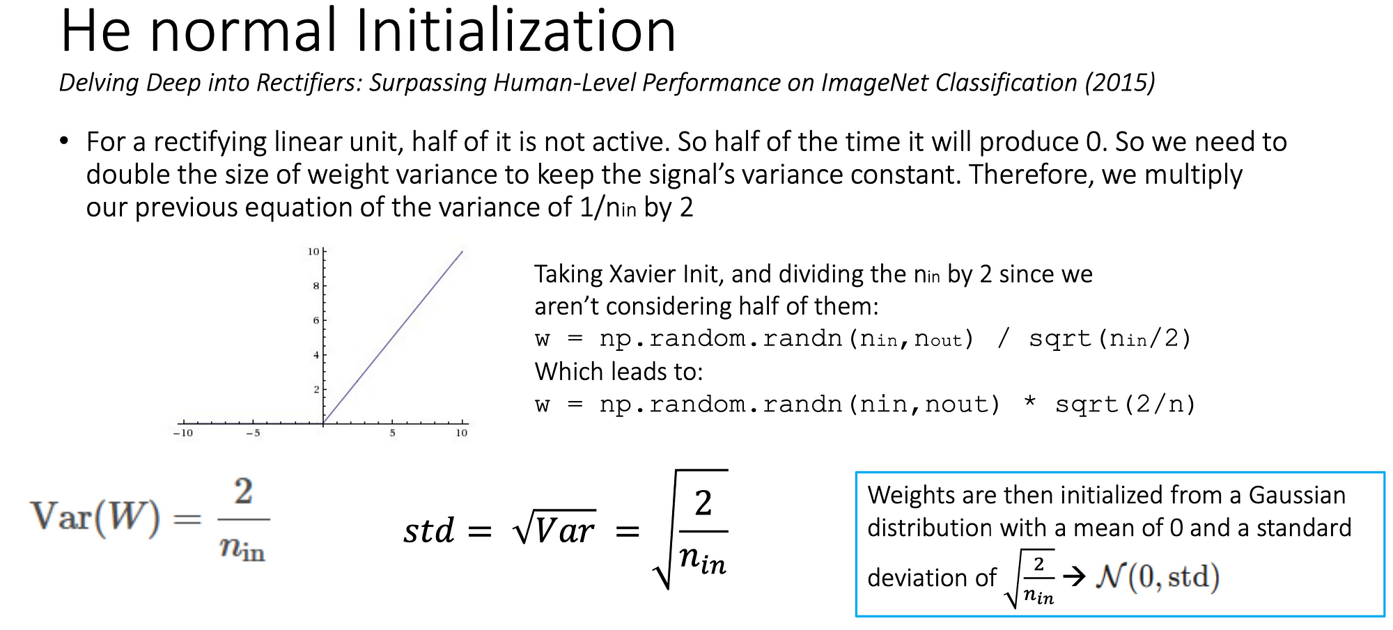
This slide illustrates the core idea of He initialization. The variance is doubled compared to a simple $1/n_{in}$ scheme to compensate for the fact that a ReLU activation zeroes out half of its inputs, thus preserving the signal's variance.

The following article provides the full mathematical proof, mirroring the structure of the Xavier derivation.

Kaiming He Initialization in Neural Networks - Math Proof

This article, also from Towards Data Science, is the companion piece to the Xavier proof and details the derivation for He initialization.

Start with the introduction and assumptions, noting the key differences for ReLU. Then, carefully follow the forward pass derivation. The critical step is where the Law of the Unconscious Statistician is used to show that E[x_k^2] = \frac{1}{2}Var[y_{k-1}], which introduces the factor of two. Finally, read the "Weight Distribution" section to see the final practical formulas for normal and uniform distributions.

Practical Implementation

Normal Distribution: We draw weights from $N (0, σ^{2})$ , where $σ^{2} = \frac{2}{n _{in}}$ .
Uniform Distribution: We draw weights from $U [- a, a]$ , where $a = \frac{6}{n _{in}}$ .

Summary and Practical Guidance

The choice of weight initialization is not arbitrary; it is a theoretically grounded decision tied directly to the activation function being used. An incorrect pairing can reintroduce the very gradient stability issues we are trying to prevent.

For a quick reference, the video below summarizes the practical rules of thumb.

Weight Initialization for Deep Feedforward Neural Networks

This short video from AssemblyAI provides a concise, practical summary of the most common weight initialization techniques.

Watch the segment on Glorot/Xavier initialization and then the segment on He initialization. Finally, review the summary table, which clearly maps the initializers to their target variances and recommended activation functions.

Here is a summary of our findings:

Initializer	Target Variance	Recommended Activation Functions
Xavier/Glorot	$\frac{2}{n _{in} + n _{o u t}}$	`tanh`, `sigmoid`, `softmax`
He	$\frac{2}{n _{in}}$	`ReLU` and its variants (Leaky ReLU, ELU, etc.)

Conclusion

In this lesson, we established the crucial role of principled weight initialization in stabilizing the training of deep neural networks. You have learned:

The Goal of Initialization: To set initial weights such that the variance of activations and gradients remains constant across layers, ensuring a signal gain of 1.
Xavier/Glorot Initialization: Derived for symmetric, zero-centered activations like tanh. It sets weight variance to $\frac{2}{n _{in} + n _{o u t}}$ as a compromise between forward and backward signal flow.
He Initialization: Derived for ReLU and its variants. It compensates for ReLU's non-symmetric nature by setting weight variance to $\frac{2}{n _{in}}$ .
The Core Principle: The choice of initializer must match the properties of the activation function to be effective.

We now have a network that is properly constructed (with non-linear activations) and properly initialized to prevent gradient instability. The next logical step is to explore how the network actually learns from data. In our next lesson, we will begin our deep dive into optimization algorithms, starting with the workhorse of modern deep learning: Stochastic Gradient Descent (SGD). We will derive it from first principles and explain its computational advantages over the batch gradient descent we've used so far.