Spin-Orbit Coupling and the Fine Structure of Hydrogen

Hello! Welcome back to our study of advanced quantum mechanics.

In our last lesson, we explored the Wigner-Eckart theorem and saw how it simplifies the calculation of matrix elements by separating geometric factors from the underlying physics. A key example was its application to scalar operators like $\hat{\vec{L}}\cdot \hat{\vec{S}}$. Today, we will see this very operator emerge as the central piece of a crucial physical phenomenon: the fine structure of the hydrogen atom.

This lesson will analyze the small corrections to the Bohr model's energy levels that arise from relativistic effects and the electron's spin. You'll learn not just what these corrections are, but where they come from and how to calculate their impact on the atom's spectrum. This is a classic application of perturbation theory and angular momentum coupling, and it represents one of the first great successes of relativistic quantum theory.

By the end of this lesson, you will be able to analyze the splitting of hydrogen's energy levels due to spin-orbit coupling and other relativistic effects, and calculate the resulting fine structure energy shifts.

1. The Physical Picture of Fine Structure

The simple model of the hydrogen atom, with Hamiltonian $H_0=\frac{{\hat{p}}^2}{2m}-\frac{e^2}{r}$, yields energy levels $E_n$ that depend only on the principal quantum number $n$. This leads to a high degree of degeneracy. However, high-resolution spectroscopy reveals that these levels are actually split into several closely spaced components. This "fine structure" is the result of three corrections to the simple Hamiltonian.

To get a feel for the experimental reality and the core idea of spin-orbit coupling, let's watch a short video.

As the video explains, the fine structure arises from three distinct physical effects, which we will treat as perturbations to $H_0$.

The Three Fine Structure Corrections

1. Spin-Orbit Coupling ($H_{SO}$): This is the most prominent term. From the electron's point of view, the proton orbits it, creating a circular current and thus a magnetic field $\vec{B}$. This internal magnetic field interacts with the electron's intrinsic spin magnetic moment ${\vec{\mu }}_s$, leading to an energy shift. The interaction Hamiltonian takes the form $H_{SO}\propto \frac{1}{r^3}\hat{\vec{L}}\cdot \hat{\vec{S}}$.

2. Relativistic Kinetic Energy Correction ($H_{rel}$): The simple kinetic energy term ${\hat{p}}^2/2m$ is a non-relativistic approximation. The correct relativistic expression for energy is $E=\sqrt{p^2{c}^2+m^2{c}^4}$. Expanding this for small velocities ($p\ll mc$) gives the first-order correction:
   $H_{rel}=-\frac{{\hat{p}}^4}{8m^3{c}^2}$

3. The Darwin Term ($H_D$): This term is a bit more abstract. It has no classical analogue and arises from the non-relativistic expansion of the Dirac equation. It can be intuitively understood as an effect of "Zitterbewegung" (trembling motion), where virtual electron-positron pair creation and annihilation cause the electron's position to be "smeared out" over a distance on the order of its Compton wavelength. This modifies the electron's interaction with the potential, particularly at the nucleus. The resulting term is:
   $H_D\propto \delta (\vec{r})$
   Because of the delta function, this term only affects states with a non-zero wavefunction at the origin, which are the s-states ($l=0$).

2. Deriving the Fine Structure Hamiltonian

Let's briefly explore the origins of these terms. A semi-classical derivation provides great physical insight into the spin-orbit term, while a more formal approach shows how all three terms emerge naturally from a single relativistic framework.

Semi-classical Derivation of $H_{SO}$

The following video derives the spin-orbit Hamiltonian using classical E&M arguments and then incorporates quantum mechanical operators. It's a great example of the "physicist's approach" you prefer. A crucial step is the inclusion of a factor of 1/2 due to Thomas Precession, a relativistic kinematic effect for accelerating frames. Without it, the result is off by a factor of two.

The result of this derivation is the spin-orbit Hamiltonian:

$$H_{SO}=\frac{e^2}{2m^2{c}^2}\frac{1}{r^3}\hat{\vec{L}}\cdot \hat{\vec{S}}$$

Formal Origin from the Dirac Equation

While the semi-classical and heuristic arguments are illuminating, it's satisfying to know that all three fine structure terms can be derived rigorously from a single starting point: the Dirac equation. A non-relativistic expansion of the Dirac equation for an electron in a central potential yields the Pauli equation plus precisely the three correction terms we've discussed.

The following resource provides a more formal and complete derivation. You have a strong enough background to appreciate this more fundamental origin.

So, our full perturbing Hamiltonian is $H_{FS}=H_{rel}+H_{SO}+H_D$. Our task is to calculate the first-order energy correction, $\Delta E_{FS}=⟨H_{FS}⟩$.

3. Calculating the Fine Structure Energy Shift

Since the unperturbed hydrogen energy levels are degenerate, we must use degenerate perturbation theory. This means we need to diagonalize the matrix of $H_{FS}$ within each degenerate subspace (i.e., for a fixed $n$).

Choosing the Right Basis

As we discussed in the last lesson, choosing a "good" basis can make the matrix diagonal from the start, saving us a lot of work. The symmetry of the operators is key.

• The uncoupled basis is $|n,l,m_l,m_s⟩$.
• The coupled basis is $|n,l,j,m_j⟩$.

$H_{rel}$ and $H_D$ are scalar operators and commute with all angular momentum operators, so they are diagonal in both bases. The trouble comes from $H_{SO}\propto \hat{\vec{L}}\cdot \hat{\vec{S}}$.

• $[\hat{\vec{L}}\cdot \hat{\vec{S}},{\hat{L}}_z]\ne 0$ and $[\hat{\vec{L}}\cdot \hat{\vec{S}},{\hat{S}}_z]\ne 0$. So, $H_{SO}$ is not diagonal in the uncoupled basis.
• $[\hat{\vec{L}}\cdot \hat{\vec{S}},{\hat{J}}^2]=0$ and $[\hat{\vec{L}}\cdot \hat{\vec{S}},{\hat{J}}_z]=0$, where $\hat{\vec{J}}=\hat{\vec{L}}+\hat{\vec{S}}$. So, $H_{SO}$ is diagonal in the coupled basis.

Therefore, the coupled basis $|n,l,j,m_j⟩$ is the correct choice to simplify our calculation. In this basis, the energy shifts are simply the expectation values of our three operators.

The Calculation

The following document provides a clear, step-by-step calculation for the expectation value of each of the three fine structure terms in the coupled basis.

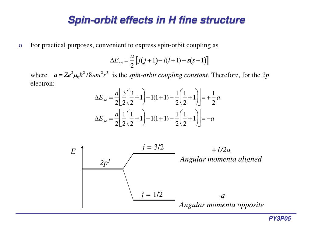
Let's summarize the key results of these calculations. The expectation value $⟨\hat{\vec{L}}\cdot \hat{\vec{S}}⟩$ in the state $|n,l,j,m_j⟩$ is:
$⟨\hat{\vec{L}}\cdot \hat{\vec{S}}⟩=\frac{{\hslash }^2}{2}[j(j+1)-l(l+1)-s(s+1)]$
Since $s=1/2$, this simplifies nicely. For a given $l$, there are two possible values for $j$: $j=l+1/2$ and $j=l-1/2$ (for $l>0$). This leads to two different energy shifts from the spin-orbit term, splitting the degeneracy.

Test your understanding!

Consider an electron in a $d$-orbital ($l=2$). What are the possible values of the total angular momentum quantum number $j$? What is the value of $⟨\hat{\vec{L}}\cdot \hat{\vec{S}}⟩/{\hslash }^2$ for each of these $j$ states?

Show answer

For $l=2$ and $s=1/2$, the possible values of $j$ are given by the triangle inequality: $|2-1/2|\le j\le 2+1/2$. So, $j=3/2$ and $j=5/2$.

We use the formula $⟨\hat{\vec{L}}\cdot \hat{\vec{S}}⟩/{\hslash }^2=\frac{1}{2}[j(j+1)-l(l+1)-s(s+1)]$.
With $l=2$ and $s=1/2$, $l(l+1)=6$ and $s(s+1)=3/4$.

• For $j=5/2$: $j(j+1)=(5/2)(7/2)=35/4$.
  $⟨\hat{\vec{L}}\cdot \hat{\vec{S}}⟩/{\hslash }^2=\frac{1}{2}[35/4-6-3/4]=\frac{1}{2}[32/4-6]=\frac{1}{2}[8-6]=1$.

• For $j=3/2$: $j(j+1)=(3/2)(5/2)=15/4$.
  $⟨\hat{\vec{L}}\cdot \hat{\vec{S}}⟩/{\hslash }^2=\frac{1}{2}[15/4-6-3/4]=\frac{1}{2}[12/4-6]=\frac{1}{2}[3-6]=-3/2$.

4. The Final Result: Hydrogen Energy Levels

When we sum the energy corrections from all three terms, something remarkable happens. After some algebra, the explicit dependence on the orbital quantum number $l$ cancels out completely!

The total first-order correction to the energy is:
$E_{FS}^{(1)}=E_n^{(0)}\frac{(Z\alpha {)}^2}{n}\left(\frac{1}{j+1/2}-\frac{3}{4n}\right)$
where $E_n^{(0)}=-\frac{1}{2}m{c}^2\frac{(Z\alpha {)}^2}{n^2}$ is the unperturbed Bohr energy and $\alpha \approx 1/137$ is the fine-structure constant.

The total energy of the state $|n,l,j,m_j⟩$ is then $E_{n,j}=E_n^{(0)}+E_{FS}^{(1)}$.

Key implications of this result:

1. The energy depends on $n$ and $j$, but not on $l$ or $m_j$.
2. The $n^2$-fold degeneracy of the Bohr model is partially lifted. States are now grouped into levels labeled by $n$ and $j$.
3. A new degeneracy appears! States with the same $n$ and $j$ but different $l$ have the same energy (e.g., the $2S_{1/2}$ and $2P_{1/2}$ states). This is a special feature of the $1/r$ potential.

This leads to the famous fine structure energy level diagram for hydrogen.

Conclusion

Today we've taken a significant step beyond the simple Bohr model of the atom. By incorporating relativistic effects and electron spin through perturbation theory, we have derived the fine structure of the hydrogen spectrum.

Key Takeaways:

• The fine structure of hydrogen is caused by three main perturbative corrections: the relativistic kinetic energy term, the Darwin term, and most significantly, spin-orbit coupling.
• Spin-orbit coupling is the interaction of the electron's spin magnetic moment with the internal magnetic field generated by the nucleus's apparent motion. Its Hamiltonian is proportional to $\hat{\vec{L}}\cdot \hat{\vec{S}}$.
• The calculation of the energy shifts is best done in the coupled basis $|n,l,j,m_j⟩$, where the spin-orbit Hamiltonian is diagonal.
• The final energy correction depends only on the quantum numbers $n$ and $j$, lifting the degeneracy in $l$ but creating a new degeneracy between states with the same $n$ and $j$ but different $l$.

Preview of the next lesson:
We have successfully analyzed the fine details of a single-electron atom. The natural next step is to consider atoms with multiple electrons. The principles of adding angular momentum become even more crucial. In the next lesson, we will introduce the LS-coupling and jj-coupling schemes, which are two important methods for classifying the quantum states and determining the term symbols for multi-electron atoms.