Testing Continuity in Metric Spaces Using Sequences

Recommended resources

The freely available resources this lesson will direct you to.

Hello! Last lesson, sequences helped distinguish convergence from the Cauchy property. Now they serve a different purpose: they let us test whether a function respects the way points approach one another. A sequence can reveal discontinuity with a single counterexample; to establish continuity, we must account for every sequence approaching the point.

This lesson develops that sequential criterion for maps between metric spaces, explains why it is equivalent to the familiar epsilon–delta definition, and uses it with ordinary, discrete, and function-space metrics.

Continuity means preserving limits

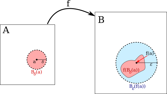
Let $f : (X, d_{X}) \to (Y, d_{Y})$ , and fix $a \in X$ . Continuity at $a$ says that for every $ε > 0$ , there is a $δ > 0$ such that

d_{X} (x, a) < δ ⟹ d_{Y} (f (x), f (a)) < ε (x \in X) .

The two distances may come from entirely different metrics. The picture shows the requirement: all inputs in a sufficiently small ball around $a$ must have outputs in the requested ball around $f (a)$ .

A ball of radius $\delta$ around $a$ in the domain maps entirely inside a ball of radius $\varepsilon$ around $f(a)$ in the codomain.

There is an equivalent test phrased entirely in terms of sequences:

Sequential criterion. The map $f$ is continuous at $a$ if and only if, for every sequence $(x_{n})$ in $X$ ,
$x_{n} \to a in (X, d_{X}) ⟹ f (x_{n}) \to f (a) in (Y, d_{Y}) .$

The word every does essential work. One well-behaved sequence cannot establish continuity, but one badly behaved sequence can disprove it. Continuity on all of $X$ means passing this test at every $a \in X$ .

Read Theorem 3.1 in Metric Spaces: Limits and Continuity. It proves both directions for arbitrary metric spaces. Give particular attention to how the converse turns a failure of the ball condition into a sequence.

Metric Spaces: Limits and Continuity

Read Theorem 3.1 for the equivalence between continuity at a point and preservation of every sequence limit. The proof is also a useful model for handling a statement with “for every sequence.”

In Theorem 3.1, begin with the statement immediately before “Proof.” In the proof’s first direction, follow the forward argument: identify where continuity supplies a ball and where convergence supplies a cutoff. Then read the contrapositive argument through the end of the proof. Focus on why choosing a point from each ball of radius 1/i produces a sequence converging to a.

The forward implication can be read as a careful matching of quantifiers. Given an output tolerance $ε$ , continuity supplies an input tolerance $δ$ . Because $x_{n} \to a$ , a cutoff $N$ puts every $x_{n}$ with $n \geq N$ inside that input ball. Their images therefore lie inside the output ball. Notice that $δ$ depends on $ε$ and $a$ , while $N$ may additionally depend on the particular sequence.

For the converse, it is clearest to reason by contrapositive. If $f$ is not continuous at $a$ , some $ε_{0} > 0$ defeats every proposed input radius. In particular, for each $n$ we can choose $x_{n} \in X$ with

d_{X} (x_{n}, a) < \frac{1}{n} but d_{Y} (f (x_{n}), f (a)) \geq ε_{0} .

The first inequality proves $x_{n} \to a$ ; the second says that the outputs never enter one fixed ball around $f (a)$ . This is why sequences are a complete test for continuity in metric spaces, not merely a convenient source of examples.

Applying the criterion: a positive proof

To prove continuity at $a$ sequentially, start with an arbitrary sequence $x_{n} \to a$ in the specified domain metric. Then show that the output distance $d_{Y} (f (x_{n}), f (a))$ tends to zero. A bound connecting output distance to input distance often does the work.

For example, give $C ([0, 1])$ , the space of continuous real-valued functions on $[0, 1]$ , the uniform metric

d_{\infty} (g, h) = t \in [0, 1] max ∣ g (t) - h (t) ∣.

Let $E : C ([0, 1]) \to R$ evaluate a function at $1/2$ : $E (g) = g (1/2)$ . If $g_{n} \to g$ in the uniform metric, then

∣ E (g_{n}) - E (g) ∣ = ∣ g_{n} (1/2) - g (1/2) ∣ \leq d_{\infty} (g_{n}, g) \to 0.

The sequence $(g_{n})$ was arbitrary, so $E$ is continuous. The estimate has a concrete meaning: if two functions are close everywhere on the interval, they must be close at the particular point $1/2$ .

Paul Minter’s Metric and Topological Spaces develops this example after defining the uniform metric. Read the short passage to see how the choice of metric makes the proof possible.

metric-and-topological-spaces-notes. ...

Read Examples 1.10 and 1.11 for a concrete continuity test on a space whose points are themselves functions. Focus on the single inequality that controls the output.

In Section 1.1, “Continuity in Metric Spaces,” on p. 7, begin at Example 1.10’s definition of the uniform metric. Read from the metric and evaluation example through the end of Example 1.11’s proof. In particular, check why a maximum over the interval bounds the difference at 1/2. You can stop before Section 1.2, “Norms.”

An output-distance estimate is powerful, but it must use the stated domain metric. Merely recognizing the same formula for a function is not enough if the metrics change.

Applying the criterion: finding a failed sequence

For a quick real-valued example, define $h : R \to R$ by $h (x) = 0$ when $x \leq 0$ and $h (x) = 1$ when $x > 0$ , using the usual metric on both spaces. At $a = 0$ , take $x_{n} = 1/ n$ . Then $x_{n} \to 0$ , but

h (x_{n}) = 1 for every n, h (0) = 0.

Thus $h$ is not continuous at $0$ . We did not have to examine every possible sequence: this one witnesses the failure.

Metrics can produce a subtler contrast without changing the underlying formula. Consider the identity map on $R$ , first from the usual metric to the discrete metric. The inputs $1/ n$ converge to $0$ as usual, but their outputs do not converge to $0$ in the discrete metric: each output remains distance $1$ from $0$ . That identity map is not continuous at $0$ .

Reverse the metrics. Any sequence converging to $a$ in a discrete metric is eventually equal to $a$ : apply convergence with a radius smaller than $1$ . Its image under any function is then eventually equal to the image of $a$ . Consequently, every function from a discrete metric space to any metric space is continuous. The contrast is about which sequences the domain regards as convergent.

Read Minter’s paired identity maps to check the direction of each claim.

metric-and-topological-spaces-notes. ...

Read Example 1.6 to see the sequential criterion distinguish two identity maps with opposite choices of domain and codomain metric.

In Section 1.1, “Continuity in Metric Spaces,” on p. 5, locate Example 1.6 immediately after Definition 1.3. Begin with the sentence assigning the Euclidean metric to X and the discrete metric to Y; continue through both identity maps. For each map, say explicitly which metric measures input convergence and which measures output convergence. Stop before Example 1.7.

Finally, a failure need not look like a single jump. Michael Penn’s video Real Analysis | Showing a function is (dis)continuous uses the function that equals $1$ on rational inputs and $0$ on irrational inputs. Watch its sequential argument for an irrational point.

Real Analysis | Showing a function is (dis)continuous.

Watch Michael Penn’s rational–irrational example to see how a dense set supplies failed sequences even when there is no isolated jump to approach.

Watch the sequence test. The argument chooses rational points approaching an irrational a. Track separately the limit of those inputs, the value of every output, and the value at a; the video leaves the rational-point case to the parallel argument.

The complementary case follows the same logic: at a rational $a$ , choose irrational $x_{n} \to a$ . Then every $f (x_{n}) = 0$ , whereas $f (a) = 1$ . At each real point there is a sequence witnessing discontinuity. The lesson is not that every approaching sequence behaves badly; it is that continuity requires none to behave badly.

Takeaways

For a map between metric spaces, continuity at $a$ is equivalent to preserving the limit of every domain sequence converging to $a$ . A positive sequential proof starts with an arbitrary such sequence and controls its output distance. A negative proof finds just one sequence whose inputs converge to $a$ but whose outputs fail to converge to $f (a)$ . In either direction, name the domain and codomain metrics before judging convergence.

Next, we will return to sequences to study compactness, where the question becomes whether every sequence in a set has a suitably convergent subsequence.