Supervised Learning: Training Fundamentals

Recommended resources

The freely available resources this lesson will direct you to.

Introduction

In our last lesson, we categorized machine learning into three main paradigms: supervised, unsupervised, and reinforcement learning. We established that supervised learning, the most common approach, is like learning with a teacher and an answer key—it uses labeled data to train a model to make predictions.

This lesson delves into the mechanics of that "teaching" process. Your goal is to understand the end-to-end training loop for a supervised machine learning model. We will dissect this process into its three fundamental components: the data used for training, the loss function that measures the model's error, and the optimization algorithm that updates the model to reduce that error. For a software developer, this is akin to understanding how a program can iteratively debug and improve itself based on a set of specifications and test cases.

The Anatomy of a Training Process

Before we dive into the details, let's look at the overall workflow. The training process for a supervised model is a cyclical loop designed to systematically minimize the model's prediction errors.

This diagram illustrates the four core stages of training a supervised model: (1) Preparing a labeled dataset, (2) Building a model and making predictions, (3) Calculating the error using a loss function, and (4) Using an optimizer to update the model. This cycle repeats until the model's performance is satisfactory.

We will now examine each of these stages in detail.

1. The Data: Providing the Ground Truth

As we covered, supervised learning requires labeled data. This simply means that for every input example, we have a corresponding correct output, or "ground-truth label." In your work as a developer, you can think of this as a collection of input-output pairs.

For a regression task (predicting a continuous value), the data might be (house_features, price).
For a classification task (predicting a category), it might be (email_text, 'spam').

The model's objective is to learn a function that can accurately map any given input to its correct output. To see how this data is structured in code, we'll look at a simple example of fitting a line to data points.

Basic training loops | TensorFlow Core

This guide from TensorFlow demonstrates the core training concepts from first principles using a simple linear model. It provides a practical, code-based perspective on the theory.

Please read the section titled "Data". Pay close attention to how the input x and the true output y are generated. The y values are created from a known line (TRUE_W * x + TRUE_B) and then a small amount of random noise is added. This simulates a real-world dataset where the underlying relationship is obscured by variability.

The key idea is that the model doesn't know the TRUE_W and TRUE_B. Its entire job is to analyze the (x, y) pairs and figure out the best possible values for its own internal weight (w) and bias (b) to approximate that hidden truth.

2. The Loss Function: Quantifying "Wrongness"

Once the model makes a prediction, we need a way to measure how far off it is from the ground-truth label. This is the job of the loss function (also called a cost function). It takes the model's prediction and the true label and computes a single number—the loss—that quantifies the error. A high loss means the prediction was poor; a low loss means it was good. The ultimate goal of training is to adjust the model's parameters to make the loss as small as possible.

Different tasks require different loss functions. Let's look at two of the most common ones.

Mean Squared Error (MSE) for Regression

For regression tasks, the standard loss function is the Mean Squared Error (MSE). It calculates the difference between the predicted value and the true value, squares it, and then averages these squared differences across all data points. Squaring the error ensures that negative errors don't cancel out positive ones and that larger errors are penalized more heavily.

Basic training loops | TensorFlow Core

The same TensorFlow guide provides a clear definition and implementation of MSE loss.

Now, read the section "Define a loss function". Notice the simplicity of the implementation: tf.reduce_mean(tf.square(target_y - predicted_y)). This directly translates the mathematical concept into code.

Cross-Entropy Loss for Classification

For classification tasks, MSE is not a good fit. Instead, we use Cross-Entropy Loss. This function is more complex but is perfectly suited for measuring the error when a model outputs probabilities for different classes (e.g., 68% chance of "Sports", 19% of "World", 13% of "Business"). It gives a high loss if the model assigns a low probability to the correct class.

The article below provides an excellent conceptual breakdown of cross-entropy loss.

How Do Neural Networks Actually Learn? A Deep Dive into Loss ...

This article breaks down the complex concepts of loss and optimization in a very accessible way.

Please read from the beginning of the article up to the end of the section "Cross-Entropy Loss Explained". Focus on these key ideas: The role of the softmax function in converting raw model outputs (logits) into probabilities. The intuition behind the cross-entropy formula: it measures the "surprise" of seeing the true outcome given the model's predicted probabilities. The loss is low if the model is confident about the correct class, and high otherwise.

3. Optimization: The Learning Algorithm

We now have a way to score our model's performance (the loss function). But how does the model actually improve? This is handled by an optimizer. The most fundamental optimization algorithm is Gradient Descent.

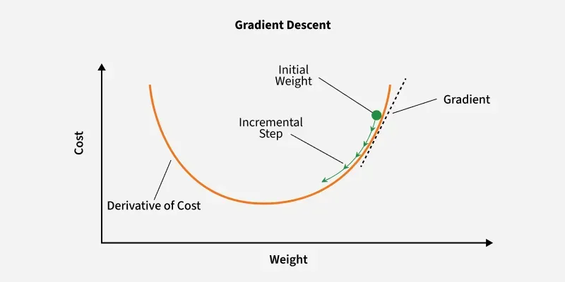
Imagine the loss function as a hilly landscape, where the elevation at any point represents the loss for a given set of model parameters (weights and biases). Our goal is to find the lowest point in this landscape—the point of minimum loss.

Gradient descent does this by taking iterative steps "downhill":

It starts at a random point in the landscape (initial random weights).
At that point, it calculates the gradient—the direction of the steepest ascent.
It then takes a small step in the opposite direction of the gradient (i.e., downhill).
It repeats this process, taking step after step, until it reaches a valley or a flat area.

The size of each step is determined by a parameter called the learning rate.

This graph illustrates the process of Gradient Descent. Starting with an initial weight, the algorithm iteratively takes small steps in the direction of the negative gradient (the steepest descent) of the cost function, moving progressively closer to the minimum cost.

The following video from StatQuest is one of the clearest explanations of gradient descent available. It builds the concept from the ground up with a simple, concrete example.

Gradient Descent, Step-by-Step

This StatQuest video masterfully explains gradient descent by first using it to optimize a single parameter and then two.

Please watch the following segments carefully: Introduction to Optimization: This sets up the problem using a simple linear regression example and introduces the sum of squared residuals as the loss function we want to minimize. Using the Derivative: This explains how the derivative (the gradient in 1D) tells us the slope of the loss curve, which indicates the direction to the minimum. Step Size and Iteration: This introduces the learning rate and shows how the new parameter value is calculated by taking a step from the old value. It visualizes the iterative process of getting closer to the minimum. General Summary: This provides a fantastic, concise summary of the entire gradient descent algorithm in six steps.

The Training Loop in Action

Now, let's put all three components—data, loss, and optimization—together into the complete training loop. This loop is the heart of training a supervised model.

Forward Pass: Feed a batch of training data through the model to get predictions.
Calculate Loss: Compare the model's predictions to the true labels using the loss function.
Backward Pass (Gradient Calculation): The optimizer calculates the gradient of the loss with respect to each of the model's parameters. This is a mathematically intensive step, but frameworks like TensorFlow and PyTorch automate it using a technique called automatic differentiation (or "autodiff").
Update Parameters: The optimizer adjusts the model's parameters by taking a small step in the direction opposite to the gradient.

This cycle is repeated many times, often for thousands or millions of iterations, over the entire dataset. Each full pass through the dataset is called an epoch.

The TensorFlow guide we looked at earlier provides a Python implementation of this exact loop.

Basic training loops | TensorFlow Core

This section shows how the concepts we've discussed are implemented in code.

Please read the section titled "Define a training loop". Focus on the train function. You will see all our components in action: model(x) makes a prediction. loss(y, model(x)) calculates the loss. t.gradient(...) computes the gradients (dw, db). model.w.assign_sub(...) updates the model's parameters.

Conclusion

In this lesson, you have deconstructed the training process of a supervised learning model. You now understand how a model uses labeled data to iteratively improve its predictions through a cycle of prediction, error measurement, and optimization.

Here are the key takeaways:

Training Data: Supervised learning relies on labeled (input, output) pairs to serve as the ground truth.
Loss Function: This function quantifies the model's error by comparing its predictions to the true labels. MSE is common for regression, and Cross-Entropy is standard for classification.
Optimization: The process of minimizing the loss function. Gradient Descent is the foundational algorithm that iteratively adjusts the model's parameters (weights and biases) by taking steps in the "downhill" direction of the loss landscape.
The Training Loop: This is the iterative cycle of making predictions, calculating loss, and updating model parameters that constitutes the "learning" process.

In our previous lessons, we built a high-level view of AI. Now, you've taken a significant step deeper by understanding the core engine that powers a vast number of machine learning models.

Next, we will shift our focus to a specific and powerful type of model that has revolutionized the field: Large Language Models (LLMs). You will learn the mechanics behind how models like GPT-4 generate human-like text by predicting tokens in a sequence.