Mathematical Derivation of Scaled Dot-Product Attention

Introduction

In our previous lesson, we established the conceptual foundation of the attention mechanism. We saw it as a powerful solution to the information bottleneck in traditional sequence-to-sequence models, enabling a model to selectively focus on relevant parts of the input at each step of output generation. This is achieved by replacing the static context vector with a dynamic one, computed as a weighted sum of all input representations.

Now, we will transition from the why to the how. This lesson delves into the mathematical core of the most prevalent attention mechanism: scaled dot-product attention. Our goal is to derive its formula step-by-step, understanding the theoretical justification for each component. By dissecting this elegant equation, you will gain a foundational understanding of the engine that powers modern Transformer architectures.

The Query, Key, and Value Framework

In our conceptual discussion, we talked about the decoder attending to the encoder's hidden states. The actual mechanism, as introduced in the "Attention Is All You Need" paper, is more general and powerful. It uses an analogy from information retrieval systems, framing attention in terms of Queries, Keys, and Values.

Instead of using raw input embeddings or hidden states directly, the model learns three distinct linear projections for each input token. This creates three new representations for each token, each with a specific role:

• Query (Q): A representation of the current token's state, essentially asking a question or "querying" the other tokens. For example, a pronoun's query might ask, "To whom or what do I refer?"
• Key (K): A representation that acts like a label or an "advertisement" for what a token contains. A noun's key might say, "I am a potential antecedent." The query will be matched against these keys.
• Value (V): A representation of the token's actual content or information. If a token is "selected" via its key, its value is what gets passed along to the output.

This separation of roles is crucial. It allows a token to advertise its relevance (Key) in a different way than it contributes its content (Value).

Mathematically, given an input matrix $X$ (where each row is a token's embedding), we generate the Q, K, and V matrices by multiplying $X$ with three distinct weight matrices, $W_Q$, $W_K$, and $W_V$, which are learned during training:

$$\begin{gathered} Q=X{W}_Q \\ K=X{W}_K \\ V=X{W}_V \end{gathered}$$

The following video provides a clear walkthrough of this initial projection step.

With this Q, K, V framework established, we can now build the full attention formula.

The Four Steps of Scaled Dot-Product Attention

The computation can be broken down into four distinct, sequential operations. We will examine each one and the mathematical reasoning behind it.

Step 1: Compute Similarity Scores with the Dot Product

The first step is to measure how much each query "matches" each key. An effective and computationally efficient way to do this is with the dot product. Given the geometric interpretation of the dot product $a\cdot b=||a||||b||\cos (\theta )$, it measures the alignment between two vectors. A large positive dot product implies the vectors point in similar directions, signaling high similarity.

We compute the dot product between every query vector and every key vector. This can be done for the entire sequence in a single, highly optimized operation: matrix multiplication.

$$\text{Scores}=Q{K}^T$$

The resulting Scores matrix contains the raw, unnormalized similarity scores. The element at position $(i,j)$ in this matrix represents the similarity between the query of the $i$-th token and the key of the $j$-th token.

Step 2: Scale the Scores

This step is the "scaled" in scaled dot-product attention and is critical for stable model training.

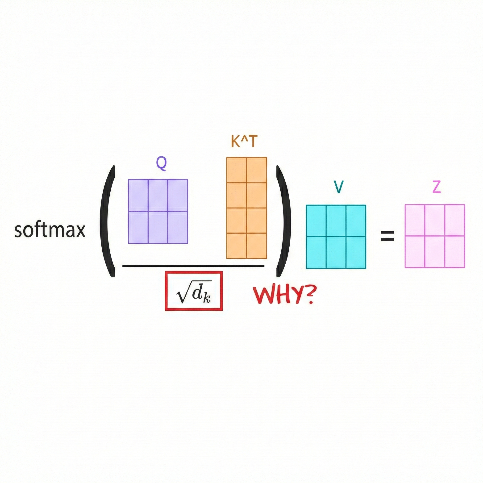
The Problem: Softmax Saturation

To understand the need for scaling, we must first consider the statistical properties of the dot product. Assume the components of your query and key vectors are independent random variables with a mean of 0 and variance of 1. The dot product of two such vectors, $q$ and $k$, of dimension $d_k$ is $q\cdot k={\sum }_{i=1}^{d_k}{q}_i{k}_i$.

From the properties of variance, the variance of this sum is the sum of the variances. Since $\text{Var}(q_i{k}_i)=\text{Var}(q_i)\text{Var}(k_i)=1\cdot 1=1$, the variance of the dot product is:

$$\text{Var}(q\cdot k)=\sum _{i=1}^{d_k}\text{Var}(q_i{k}_i)=d_k$$

The standard deviation is therefore $\sqrt{d_k}$. This means that as the dimension $d_k$ of the keys and queries increases, the variance of the dot products also increases, leading to scores with larger magnitudes.

These large scores are then fed into a softmax function (our next step). The softmax function, $e^{z_i}/{\sum }_j{e}^{z_j}$, is sensitive to large inputs. If one score is significantly larger than others, the softmax output will be extremely "peaky"—approaching a one-hot distribution where one token gets an attention weight near 1 and all others get weights near 0. This is called softmax saturation.

In this saturated regime, the gradients become vanishingly small for all non-maximal inputs. The model effectively stops learning, as there is no gradient signal to update the weights.

The Solution: Variance Normalization

To counteract this, the original authors proposed a simple and elegant solution: divide the scores by the standard deviation, $\sqrt{d_k}$.

$$\text{Scaled Scores}=\frac{Q{K}^T}{\sqrt{d_k}}$$

This step normalizes the scores to have a variance of 1, regardless of the dimension $d_k$. This keeps the inputs to the softmax function in a well-behaved range, preventing saturation and ensuring that gradients can flow properly during training.

The following resources provide a detailed statistical derivation and intuition for this crucial step.

Step 3: Compute Attention Weights with Softmax

With the scores appropriately scaled, we apply a row-wise softmax function to convert them into a probability distribution.

$$A=\text{softmax}\left(\frac{Q{K}^T}{\sqrt{d_k}}\right)$$

The resulting matrix $A$ is the attention weight matrix. Each row $A_i$ is a probability distribution that sums to 1. The value $A_{ij}$ represents the amount of attention the $i$-th token should pay to the $j$-th token. The softmax sharpens the distribution, assigning exponentially higher weights to tokens with higher similarity scores.

Step 4: Compute the Output as a Weighted Sum of Values

The final step is to use the attention weights to create a weighted sum of the Value vectors.

$$\text{Output}=AV=\text{softmax}\left(\frac{Q{K}^T}{\sqrt{d_k}}\right)V$$

The output for the $i$-th token is a new vector computed by summing all value vectors $V_j$, weighted by their corresponding attention scores $A_{ij}$. This new vector is a context-aware representation of the token, containing information blended from across the entire sequence, precisely controlled by the learned attention weights.

The Complete Formula

By combining these four steps, we arrive at the complete formula for scaled dot-product attention:

$$\text{Attention}(Q,K,V)=\text{softmax}\left(\frac{Q{K}^T}{\sqrt{d_k}}\right)V$$

This single, compact equation elegantly captures the entire process: measuring similarity, stabilizing the computation, converting scores to probabilistic weights, and aggregating information. Crucially, every operation within this formula—matrix multiplication, scaling, and softmax—is differentiable. This allows gradients from a downstream loss function to flow back through the entire mechanism, enabling the weight matrices $W_Q,W_K,W_V$ to be optimized end-to-end via standard backpropagation.

Conclusion

In this lesson, we have mathematically deconstructed scaled dot-product attention, the fundamental building block of the Transformer. We moved beyond the high-level concept of attention and derived its specific implementation, understanding the theoretical necessity of each component.

The key takeaways are:

• Q, K, V Framework: Inputs are projected into three distinct roles—Query, Key, and Value—allowing for a flexible and powerful attention mechanism.
• Similarity Scores: The dot product $Q{K}^T$ provides an efficient and effective measure of similarity between queries and keys.
• The Scaling Factor: Dividing by $\sqrt{d_k}$ is a crucial step for numerical stability. It normalizes the variance of the dot products, preventing the softmax function from saturating and causing vanishing gradients, thus enabling the training of deep models.
• The Final Output: The attention weights, derived from the softmax of the scaled scores, are used to compute a weighted sum of the Value vectors, producing a context-enriched representation for each token.
• Differentiability: The entire mechanism is fully differentiable, allowing for end-to-end training with gradient-based optimization.

You now understand how attention is calculated for a single "head." However, a single attention mechanism might be forced to average its focus. What if we want the model to pay attention to different things simultaneously—for instance, attending to syntactic dependencies in one way and semantic relationships in another? This is the motivation for our next topic: multi-head attention.