Recommended resources
The freely available resources this lesson will direct you to.
Hello. The previous lesson treated each raw pixel value as a noisy measurement and used repeated exposures to separate shot noise, read noise, and persistent pixel variation. Now there is a different limitation: even a perfectly noiseless color-filter-array pixel measures only one spectral band at its location. The other color values must be inferred.
In about 40–45 minutes, you will model a Bayer measurement, reconstruct a full-color image using both straightforward and edge-aware interpolation, and distinguish errors caused by inadequate sampling from errors introduced by reconstruction. That distinction matters whenever a camera photographs fine fabric, architecture, or other nearly periodic detail.
What a color-filter array actually measures
A single image sensor can place red, green, or blue filters over different photosites. In a Bayer array, each repeating two-by-two cell contains two green sites, one red, and one blue. One possible orientation is
| Even column | Odd column | |
|---|---|---|
| Even row | R | G |
| Odd row | G | B |
The orientation can be shifted or rotated; the reconstruction software must know which sites measured which band. Green has twice as many sites as either red or blue. This gives the array denser sampling for much of the image detail that contributes to perceived brightness, though green is not itself luminance.
Russ Palum’s conference paper, Image Sampling with the Bayer Color Filter Array, connects this layout to a concrete reconstruction method. Read its opening and interpolation discussion before examining the image below.
[PDF] Image Sampling with the Bayer Color Filter Array
Read Russ Palum’s account for the engineering reason behind the Bayer layout and for a comparison of blockwise and adaptive reconstruction.
On p. 239, in “Introduction,” read the CFA setup, ending with the explanation of the two green samples. Continue from the paragraph beginning “The simplest way to interpolate the Bayer CFA” through the black-and-white edge example in Figure 4 on p. 240: block artifacts. Then read “Adaptive Interpolation” and “Some of the Details” on p. 240, from the green-first description through Figure 6 and the resulting RGB image: adaptive reconstruction. Focus on why the method estimates green first and then interpolates red-minus-green and blue-minus-green.

It helps to write down what is—and is not—in that raw mosaic. Let , , and denote the values that the camera’s three filtered responses would produce at image location , after spatial blur and pixel integration. They are camera-dependent spectral-band measurements, not a complete spectrum of the incoming light. If , , and are binary masks marking the filter at each site, an offset-corrected raw observation can be modeled as
The noise term recalls the previous lesson. Crucially, there is one observation for three unknown band values at each site. Demosaicing is therefore an underdetermined reconstruction problem. It becomes possible only by using information from neighboring sites and assumptions about how images vary across space.
Reconstructing the missing values
Begin with a local-smoothness assumption. At a red site, estimate missing green from its four neighboring green sites and missing blue from its four diagonal blue sites. At a green site, the missing red and blue values can be estimated from the two nearest samples of each respective band; which pair is horizontal depends on that site’s position in the Bayer pattern. At a blue site, exchange the roles of red and blue.
For example, suppose a red site measures , its four neighboring green measurements average , and its four diagonal blue measurements average . This elementary interpolation assigns it an estimated color vector
Only the red entry was measured there. The other two are estimates. Applying analogous rules everywhere produces three full-size planes, but averaging across a sharp boundary mixes opposite sides of that boundary. Palum’s simplest two-by-two block method is more severe still: it copies a block’s sparse color readings into multiple output positions. At a neutral black-and-white edge, the filter positions can then make one side appear cyan or yellow even though the scene has no colored edge.
An edge-aware method asks a better question: in which direction is it safer to interpolate? At a red or blue site, compare the green values on its left and right with those above and below. If the horizontal pair is much more similar than the vertical pair, interpolate green horizontally; if the vertical pair is more similar, interpolate vertically. This is an estimate of local structure, not a guarantee: repeated stripes, fine corners, and noisy readings can make a gradient test choose the wrong direction.
The second improvement uses correlation between color planes. After estimating a full green plane, form known color differences at measured red and blue sites, interpolate those differences, and add green back:
This assumes color differences usually vary more slowly than brightness detail. If a bright-to-dark edge affects all three bands similarly, the reconstructed channels can share the relatively well-sampled green edge instead of acquiring separate, misaligned edges. The assumption can fail at an abrupt colored boundary. Also, Palum’s observation that a neutral region has zero color differences presumes appropriately normalized channel responses; unadjusted raw R, G, and B readings need not be equal under neutral light.
For a second perspective, read the focused portions of Gunturk and colleagues’ Demosaicking: Color Filter Array Interpolation. It is a survey rather than a prescription for one “best” algorithm; here its value is making the assumptions behind edge-directed and cross-channel interpolation explicit.
Demosaicking: Color Filter Array Interpolation
Read Gunturk and colleagues’ IEEE Signal Processing Magazine article to compare two families of reconstruction assumptions with Palum’s green-first method.
On pp. 45–46, under “DEMOSAICKING METHODS” and “HEURISTIC APPROACHES,” read “EDGE-DIRECTED INTERPOLATION” from its comparison with nonadaptive interpolation through the directional example in Figure 3: edge direction. Then read “CONSTANT-HUE-BASED INTERPOLATION” from its opening assumption through the discussion accompanying Figure 5: color correlation. Notice that channel ratios and channel differences are related approaches but make different assumptions when illumination varies.
These methods trade one kind of error for another. A smooth interpolator may suppress spurious color but blur genuine detail. An aggressive edge-preserving method may retain detail yet amplify a mistaken directional decision. Neither can determine an arbitrary missing color pattern from one mosaic without additional assumptions.
When the measurements themselves are ambiguous
Demosaicing is not the only source of false detail. Before reconstruction, the optics form a continuous image and each photosite integrates light over an area. The CFA then samples different spectral bands on different spatial grids. If the image contains detail too fine for a grid, distinct patterns can yield the same samples: aliasing has occurred.
This video derives that ambiguity using replicated spectra. Watch the derivation and its discussion of optical and pixel-area filtering. Treat its suggestion that filtering can make images entirely alias-free as an ideal band-limiting argument; real optical responses do not generally have a perfect cutoff.
Sampling Theory and Aliasing | Image Processing II
Watch “Sampling Theory and Aliasing” from First Principles of Computer Vision for the Fourier-space explanation of why interpolation cannot uniquely undo undersampling.
Watch spectral replicas, from the impulse-train model through the overlap that makes reconstruction ambiguous. Then watch physical filtering for the effects of finite pixel area and an optical low-pass filter. Relate both to the image formed on a CFA sensor, where the color bands occupy different sampling grids.
Palum then extends the sampling argument to Bayer geometry. His diagrams are particularly useful because a single Nyquist number cannot describe every color and direction in this two-dimensional array.
[PDF] Image Sampling with the Bayer Color Filter Array
Return to Palum’s paper to see how the red, blue, and green sampling grids differ—and why the orientation of fine detail matters.
On pp. 240–241, in “Spatial Frequency, Nyquist Frequency, and Sampling Frequency,” begin with the sampling condition. Continue through “Nyquist Domain Graph” on pp. 241–242, then “Bayer Pattern” and “Green Array” on pp. 242–244, ending at the Bayer grids. Concentrate on Figures 13 and 16: compare the red/blue domain with the green domain, and compare horizontal or vertical detail with diagonal detail. Some equations in the extracted PDF text render poorly; use the figures and the stated pixel spacings.
Let the underlying photosite pitch be . Along a row that contains red samples, their spacing is , so the red sampling frequency along that row is and its one-dimensional Nyquist frequency is . Blue has a similarly spaced grid. Green sites form a staggered checkerboard grid; its two-dimensional sampling domain differs both from red/blue and from an unfiltered square array. In Palum’s diagrams, green supports higher horizontal and vertical frequencies than red or blue alone, but its limit changes with orientation.
A numerical example makes the danger tangible. Suppose horizontal brightness stripes contain a component at cycles per . Red sites along one of their rows sample at samples per . In that row’s red samples, the component is indistinguishable from a much slower variation at
That false low frequency corresponds to a broad variation with period , rather than the original fine stripes. Other samples may help an algorithm infer the true structure if its cross-channel assumptions hold, but interpolation of those red samples alone cannot reveal which frequency generated them. Optical blur, pixel integration, and an optical low-pass filter can attenuate troublesome high frequencies before sampling; stronger attenuation also sacrifices some fine detail.
Reading the artifacts in a photograph
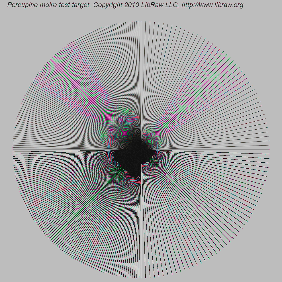
The dense spokes provide many orientations and spatial frequencies in one field. In a controlled camera comparison, you would retain the raw mosaic, vary only the reconstruction method, and inspect the same crop at a known display scale. That separates observations more reliably than assigning every colored ripple to “bad demosaicing.”
Three signatures are worth distinguishing:
| Visible signature | Likely mechanism | Useful diagnostic |
|---|---|---|
| Broad, slowly varying bands over fine repetitive detail | Moiré: fine structure has aliased into a lower spatial frequency | Check whether its spacing or orientation changes as the pattern’s scale relative to the pixel grid changes. |
| Colored fringes or false colors on fine neutral detail | CFA bands have sampled the structure differently; reconstruction has interpreted the mismatch as color | Check the raw mosaic and compare reconstructions. If the color is absent from the subject, it is not a faithful color estimate. |
| Alternating, jagged color or brightness along an edge—a zipper pattern | Interpolation has made inconsistent local decisions near the edge | Compare a simple interpolator with an edge-aware one at the same raw samples. |
These categories interact. Aliasing is a measurement ambiguity created at sampling; a demosaicing algorithm can make it conspicuous, hide it, or create additional edge artifacts. Once two input patterns have produced indistinguishable samples, no single-frame algorithm can guarantee recovery of the correct one without further information. Conversely, if two algorithms produce different zipper patterns from the same raw data, those differences implicate reconstruction rather than a change in the optical measurement.
The article by Gunturk and colleagues evaluates methods on more than one image-quality measure. Its examples are a useful warning against selecting an algorithm solely by average numerical error.
Demosaicking: Color Filter Array Interpolation
Return to the article’s comparison to connect measurable reconstruction error with the appearance of aliasing and zipper artifacts.
On p. 51, under “COMPARISON,” read from the paragraph defining the zipper-effect measure through the explanation of Table 1: zipper measurement. Then read the paragraphs beginning “The numbers can only provide part of the overall story” through the comparison of the lighthouse and boat images: visible artifacts. Compare Figures 10 and 11 if they are legible, particularly the fine fence and differently oriented lines.
An engineering response depends on the diagnosis. If fine scene detail is aliasing at capture, reducing its image-plane contrast before sampling—through optical low-pass filtering or other appropriate optical choices—addresses the cause, at a sharpness cost. If the samples adequately represent the detail but reconstruction damages an edge, changing the interpolation rule may help without changing hardware. If noisy raw samples are triggering unstable edge choices, suppressing noise may help, but excessive smoothing can remove the very structure the algorithm is meant to preserve.
Conclusion
A Bayer sensor records a mosaic of single-band measurements, not a full RGB vector at every photosite. Demosaicing fills the missing entries by assuming local smoothness, edge continuity, or correlation between color bands. Green-first, color-difference interpolation often preserves shared detail better than independent channel averaging, but its assumptions can fail.
The central diagnostic distinction is sampling versus reconstruction. Aliasing and moiré arise when fine optical detail becomes ambiguous on a sampling grid; false color and zippering describe ways that ambiguity or interpolation choices appear in the output. The next lesson follows these reconstructed, still camera-dependent measurements through calibration, white balance, color transformation, tone mapping, and output encoding.